Recombination#

The EPOCH collisional ionisation and recombination package allows for three types of recombination between an incident electron and a target ion: dielectronic, radiative, and three-body recombination. The method is described in a paper which, at the time of writing this documentation, is still under review. I will (ambitiously) refer to this paper as Morris (2025), “Recombination effects in laser-driven acceleration of heavy ions”.

The ionisation/recombination package subtracts the recombination rate from the ionisation rate, and only the dominant process is applied. If recombination triggers, the macro-electron is removed from the simulation, and a macro-ion is moved to a species with a higher charge-state. To conserve momentum in the simulation, the real electron momentum is added to the real ion momentum in the final ion macro-particle.

Recombination rates are described in terms of the parameter \(\alpha\), with units [m³/s]. The actual rate of triggering recombination for a given incident electron is \(n_i \alpha\), where \(n_i\) is the background ion number density. We evaluate \(\alpha\) in the ion-rest-frame, then transform this back to the simulation frame when calculating recombination probabilities. This page will describe the recombination rates of each process, the methods used to transform \(\alpha\) between frames, and will provide basic recombination examples.

Dielectronic recombination#

Dielectronic recombination describes the two-step process where an incident electron is first captured to an excited state of an ion, and then de-excites through photon emission to become a bound electron. The process is described in Fritzsche (2021) Astronomy & Astrophysics 656, A163, and a method for calculating these rates with the JAC code is also provided in this paper.

The cross-section for dielectronic recombination is strongly peaked near the resonance, and the probability of a single macro-electron having this energy is very low. Instead, the rates are obtained through calculating the fraction of electrons which would hit this cross-section, assuming a thermal, Maxwellian electron population characterised by some temperature \(T_e\).

While some evaluations of \(\alpha(T_e)\) have been performed using the JAC code, these calculations are computationally demanding. Currently, EPOCH only uses JAC data for the \(\text{Au}^{69+}\rightarrow \text{Au}^{68+}\) and \(\text{Au}^{68+}\rightarrow \text{Au}^{67+}\) transitions, which were calculated for use in Morris (2025). The remaining data-points come from the online FLYCHK tables, detailed in Chung (2005) High energy density physics 1, 3.

Dielectronic recombination rates are read to the code from file, and are found in tables/dr_rates. The table filenames are written in the format dr_ZZ.dat, where ZZ is replaced with a two digit atomic number (with leading 0 where appropriate). A subset of values from these tables is shown here, for carbon:

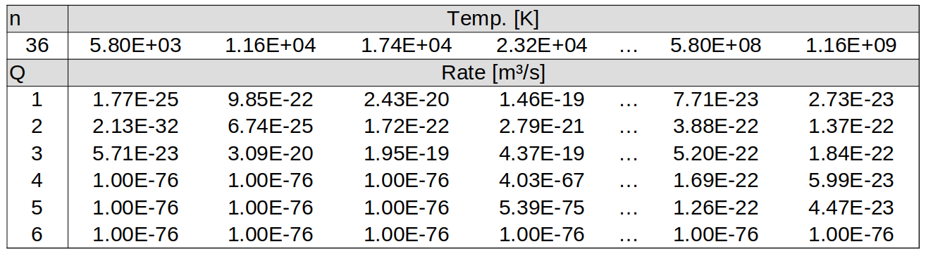
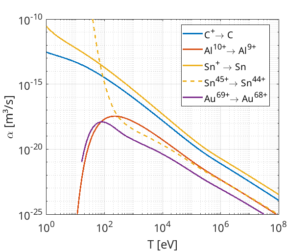
Sample of dielectronic recombination table for carbon

These tables contain a set of \(n\) temperature values, with the recombination \(\alpha\) at each temperature calculated for each ion charge-state, \(Q\). The charge-states listed refer to the ion charge before recombination occurs. A sample of \(\alpha\) rates for various ions is provided here:

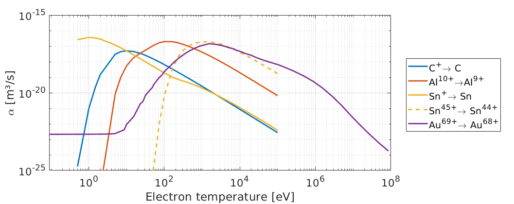
Dielectronic recombination rates for various ion transitions

The FLYCHK tables have data on dielectronic recombination rates up to gold, over a temperature range which varies between 0.5 eV and 100 keV. The Au transition in this figure was calculated using JAC, which extends the temperature domain. EPOCH uses the last tabulated value for temperatures which exceed the table range, which is expected to be an acceptable extrapolation. Ionisation is assumed to dominate recombination at high temperatures, so the exact form of recombination here should be unimportant.

Radiative recombination#

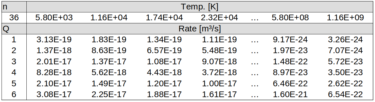
Radiative recombination refers to the inverse process of ionisation through direct absorption of a photon. The calculation of radiative recombination rates is described in Chung (2005) High energy density physics 1, 3, where detailed balance is used to convert photo-ionisation rates to the inverse recombination process. The rates are tabulated by FLYCHK using a similar format to dielectronic recombination, and these rates have been copied to the EPOCH files tables/rr_rates/rr_ZZ.dat. These files follow the same format as for dielectronic recombination, and a subset of radiative recombination rates is shown here, for carbon:

Sample of radiative recombination table for carbon

As in the dielectronic recombination case, we can compare the radiative recombination rates of different ions against each other, by plotting the values in these tables:

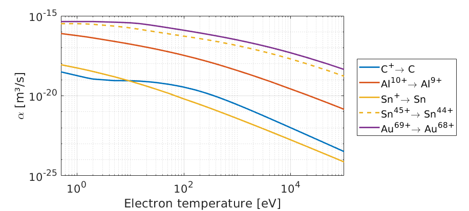
Radiative recombination rates for various ion transitions

Since radiative recombination rates are restricted to the values given by FLYCHK, tables only go up to gold, and they give temperatures between 0.5 eV and 100 keV. The code uses the last tabulated value beyond these temperatures, as in the case of dielectronic recombination. The exact form of high temperature recombination is expected to be unimportant, as ionisation should dominate above 100 keV temperatures.

Three-body recombination#

A model for three-body recombination has been derived following the theory presented in Kremp’s (2005) textbook: “Quantum statistics of nonideal plasmas”. The implementation of this model into the EPOCH code is discussed in Morris (2025). Three-body recombination refers to the inverse process of collisional ionisation, where electrons collide near ions, and one loses sufficient energy to be captured by the ion. In Kremp (2005) Eq. (2.232), the change in electron number density due to three-body recombination is written as:

\( \left(\frac{dn_e}{dt}\right)_{3BR} = \sum_j\left( -n_e^2 n_i \beta_j \right)\)

where the sum is performed over all atomic levels \(j\). For comparison to dielectronic and radiative recombination, the \(\alpha\) rate here is equivalent to \(n_e \beta_j\). An expression for \(\beta_j\) is provided in Kremp (2005) Eq. (8.47)

\( \beta_j = g_j \Lambda_e^3 \alpha_j e^{I^\text{eff}_j / k_B T_e}\)

where \(\alpha_j\) is the collisional ionisation rate for state \(j\) of the recombined species, \(\langle v_e \sigma_j\rangle\). Here, \(v_e\) is the incident electron velocity, \(\sigma_j\) is the collisional ionisation cross-section associated with ejecting a bound electron from state \(j\), and the average is performed over all local free electrons. The thermal wavelength \(\Lambda_e\) is related to the electron temperature, \(T_e\), and is given by Kremp (2005) eq. (2.18)

\(\Lambda_e = \sqrt{\frac{2\pi \hbar^2}{m_e k_B T_e}}\)

The parameter \(g_j\) refers to the statistical weight of level \(j\), which is characterised by quantum numbers \(n\) and \(l\). We will take this to be the degeneracy of state \(j\), which is \(2(2l + 1)\).

Finally, \(I^\text{eff}_j\) is the effective ionisation energy of a bound electron in state \(j\) of the recombined ion. The “effective” label refers to how the ionisation energy drops with increasing plasma density, as shown in Kremp (2005) Fig. 2.6.

Since we are creating a model for a PIC simulation, let us make two approximations. Firstly, PIC codes model weakly coupled plasmas, so let us ignore the ionisation-energy-shift. Hence, \(I^\text{eff}_j \approx I_j\), where \(I_j\) is the energy required to ionise an electron in shell \(j\). Secondly, since we aren’t tracking excited states, let us assume all transitions occur between ground-states. By inspecting how ground-state configurations change between successive ion charge-states, we can determine the shell which ejects a bound electron - let this shell be the only shell considered for \(j\). Hence, the three-body recombination rate for an ion of charge-state \(Q\) is:

\(\alpha^\text{3BR}_Q = 2(2l+1) n_e \Lambda_e^3\alpha^{\text{CI},nl}_{Q-1} e^{I_{Q-1}/k_B T_e}\)

where \(I_{Q-1}\) is the ionisation energy in the ion of charge-state \((Q-1)\) (taken from NIST), and \(nl\) are the quantum numbers related to the shell which ejects the bound electron in the ground-state transition from \((Q-1)\) to \(Q\). The term \(\alpha^{\text{CI},nl}_{Q-1}\) describes the collisional ionisation rate using the cross section corresponding to a bound electron in shell \(nl\) of the ion with charge-state \((Q-1)\).

The presense of \(n_e\) in the \(\alpha^\text{3BR}_Q\) expression makes this rate tricky to calculate in EPOCH, as the electron species is an incident species, not a background species. Instead, the code will loop over all species marked with the identify:electron key (or equivalent electron species identity), and save the electron number density as a multi-species derived array. If two or more electron species are present, the full \(n_e\) is used for both. This ensures two identical electron species have the same rate as a single physically-equivalent electron species, such that the physics doesn’t change based on how macro-electrons are distributed between species.

The three-body recombination implementation is simplified by creating a table to contain \(\sigma^{\text{CI},nl}_{Q-1}\) values as a function of incident kinetic energy, which are used to calculate \(\alpha^{\text{CI},nl}_{Q-1}\). At the start of the simulation, species properties are loaded for the \((Q-1)\) ion species, and the cross-sections are calculated as they are in the collisional ionisation process - but only for the outer-most bound electron in state \(nl\). An example of this table for Sn (recombination from \(\text{Sn}^+\)) is given here:

Sample of outer-shell collisional ionisation cross-section table for tin

Incident kinetic energy values in this table have been written in eV for easy viewing, but the code stores them in J.

In the code, \(\alpha^{\text{CI},nl}_{Q-1}\) is calculated in the ion-rest-frame by pairing macro-electrons with local macro-ions, transforming the electron momentum to the ion-rest-frame, and calculating \(\langle \sigma^{\text{CI},nl}_{Q-1}(v_e) v_e\rangle\) in each cell using the saved \(\sigma^{\text{CI},nl}_{Q-1}\) tables. If we instead assume a Maxwellian distribution of electrons (Maxwell-Juttner for relativistic temperatures), we can calculate a theoretical \(\alpha^{\text{CI},nl}_{Q-1}\) value by sampling \(v_e\) from this thermal distribution. This allows us to model the three-body recombination rate \(\alpha^\text{3BR}_Q\), for some choice of electron number density, which has been done in this figure:

Three-body recombination rates for various materials, in quasineutral plasma with ion number density 6.0e28/m³

Here, we assume the plasma has an ion density of \(n_i=6\times10^{28} \text{ m}^{-3}\), which roughly corresponds to a solid-density plasma. The electron density has been chosen to make the target quasineutral \(n_e\approx Q n_i\), where \(Q\) is the ion-charge-state before recombination.

Ion-rest-frame transformations#

In dielectronic, radiative, and three-body recombination, the rates are evaluated in the ion-rest-frame, and are then transformed back to the simulation frame for the probabiltiy calculation. All 3 processes require the temperature, and three-body recombination needs the electron number density too. Hence, we require transformations for density, temperature, and the \(\alpha\) rate.

For temperature, we may follow the procedure in Morris (2025) Appendix A. Firstly, assume that recombination is only important at low, non-relativistic temperatures, where we can equate the thermal energy to kinetic energy as:

\( T_e = \frac{\langle p^2\rangle}{3 m_e k_B} \)

where the average is performed over all local electrons. Let us also assume that this non-relativistic electron population is isotropic, which allows us to define an arbitrary co-ordinate system. Let us use a system where a Lorentz boost in the \(x\) direction transforms us to the ion-rest-frame. Here:

\(p_x' = \gamma_i \left(p_x - \beta_i \frac{E_e}{c} \right)\)

\(p_y' = p_y\)

\(p_z' = p_z\)

where \(E_e\) is the electron total energy, \(\gamma_i\) and \(\beta_i\) are the ion Lorentz factor and \(c\)-normalised velocity respectively, and \((')\) marks quantities evaluated in the ion-rest-frame.

By writing the temperature in the ion-rest-frame as

\(T_e' = \frac{\langle \left(p_x'\right)^2\rangle + \langle \left(p_y'\right)^2\rangle + \langle \left(p_z'\right)^2\rangle}{3 m_e k_B}\)

and using the isotropic electron approximation to write \(\langle p^2\rangle = 3\langle p_i^2 \rangle\) for arbitrary direction \(i\), we can write

\(T_e' = \frac{1}{3 m_e k_B} \left(\left( \frac{1}{3}\gamma_i^2 + \frac{2}{3} + \gamma_i^2 \beta_i^2\right)\langle p^2\rangle + \left(\gamma_i\beta_i m_e c\right)^2 - \frac{2\beta_i\gamma_i^2}{c}\langle p_x E_e\rangle \right)\)

Hence, the temperature in the ion-rest-frame may be estimated by pre-calculating the simulation-frame averages \(\langle p^2 \rangle\) and \(\langle p_x E_e \rangle\) at the start of each step, and using the current ion \(\gamma_i\).

For number density, let us recall the expressions for time dilation and Lorentz contraction:

\(\Delta t = \gamma_i \Delta t'\)

\(\Delta x = \frac{1}{\gamma_i} \Delta x'\)

Suppose a volume of \(\Delta x \Delta y \Delta y\) in the simulation frame contained \(N\) particles. There would still be \(N\) particles in the ion-rest-frame, but now the volume would be \(\Delta x' \Delta y' \Delta z'\). Using the Lorentz contraction formula, we can therefore write:

\(n_e' = \frac{N}{\Delta x' \Delta y' \Delta z'} = \frac{1}{\gamma_i} n_e\)

Finally, to get the \(\alpha\) transformation, we assert the probability of recombination must be the same in both-frames, since different frames cannot contain different numbers of recombined particles. Hence:

\(\alpha \Delta t n_i = \alpha' \Delta t' n_i'\)

Using the density transform and time dilation formulae, we can provide a transformation from the ion-rest-frame rate to the simulation-frame rate

\(\alpha = \alpha' \frac{1}{\gamma_i^2}\)

Example: Dielectronic and radiative recombination#

While the rates of dielectronic and radiative recombination are quite similar, three-body-recombination will dominate in different regimes. Hence, let us test these processes separately. This example will look at the rate of \(\text{Sn}^{45+}\) recombination in the presence of a mono-energetic 10 keV electron population. Collisional ionisation and three-body recombination have been switched off.

Since temperature in EPOCH is related to the average squared momentum in the cell, \(\langle p^2 \rangle\), it is simple to deduce that the temperature of our 10 keV electron bunch is 6.7 keV. This temperature corresponds to rates of \(6.4\times 10^{-18} \text{ m}^3\text{s}^{-1}\) and \(1.9\times 10^{-18} \text{ m}^3\text{s}^{-1}\) for dielectronic and radiative recombination respectively. In the code, the recombination rate is taken to be the sum of these two rates. Note that this is not how the recombination package is intended to be used, as a mono-energetic bunch of drifting electrons is clearly not an isotropic Maxwellian distribution. We simply use a drifting bunch here as it simplifies the rate calculation, allowing us to model the expected behaviour more easily.

A solid density of \(6\times 10^{28} \text{ m}^{-3}\) was used for the \(\text{Sn}^{45+}\) ion species, and the electron species was initialised with a neutralising density. Macro-electrons had their charge set to 0, such that their motion generated no currents on the grid, and so their momentum remained fixed until recombination. This allowed a simple model to be developed for estimating the number of \(\text{Sn}^{45+}\) ions as a function of time:

\(\frac{d n_i}{d t} = - n_e(t) n_i(t) \alpha\)

\(\frac{d n_e}{d t} = - n_e(t) n_i(t) \alpha\)

where \(\alpha\) is constant due to the mono-energetic electrons present. The results of EPOCH were compared against this simple model, which yielded the population evolution figure shown here:

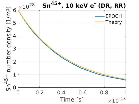
Falling density of a tin-45 species over time, due to dielectronic and radiative recombination with a 10 keV e- species

The resultant plot shows a good agreement against the simple ion-population model. The simulation supporting this figure was performed using the following input deck:

begin:control
  nx = 10
  x_min = 0
  x_max = 0.2e-6
  t_end = 100.0e-15
  verbose = 2
  stdout_frequency = 1
end:control

begin:boundaries
  bc_x_min = periodic
  bc_x_max = periodic
end:boundaries

begin:physics_package
  process = collision_ionise_recombine
  incident = Electron
  background = Tin45
  recombine_to_species = Tin44
  use_dielectronic_recombine = T
  use_radiative_recombine = T
  use_three_body_recombine = F
  use_collision_ionise = F
end:physics_package

begin:species
  name = Electron
  mass = 1
  charge = 0
  drift_x = 5.4291e-23
  rho = 45 * 6.0e28
  npart = 1000 * nx
end:species

begin:species
  name = Tin45
  atomic_number = 50
  charge = 45
  mass = 216395 - 45
  rho = 6.0e28
  npart_per_cell = 1000
  immobile = T
end:species

begin:species
  name = Tin44
  atomic_number = 50
  charge = 44
  mass = 216395 - 44
  immobile = T
end:species

begin:output
  name = rst
  nstep_snapshot = 10
  rolling_restart = F
  dump_first = T
end:output

Example: Three-body recombination#

This example shows the time evolution of a \(\text{Sn}^+\) species, surrounded by an electron species which can trigger three-body recombination to a Sn state. A drift momentum is applied to the electron species, equivalent to a kinetic energy of 1.1 keV, and a temperature of around 750 eV. Both \(\text{Sn}^+\) and \(e^-\) species start with a number density of \(6\times 10^{28} \text{ m}^{-3}\), providing an initial \(\alpha\) value of around \(3.6 \times 10^{-16} \text{ m}^3\text{s}^{-1}\).

While macro-electrons are initialised with some momentum, they are set immobile in this simulation, so their position and speed will not be updated by the standard particle pusher. This keeps their speed fixed, so the \(\alpha\) rate only varies with the electron number density. While dielectronic and radiative recombination have \(\alpha\) rates independent of \(n_e\), three-body recombination includes this dependence, so the expected evolution of the ion and electron species is:

\(\frac{d n_i}{d t} = - n_e(t) n_i(t) \alpha(n_e)\)

\(\frac{d n_e}{d t} = - n_e(t) n_i(t) \alpha(n_e)\)

Here, \(\alpha(n_e)\) only considers contributions from the three-body recombination process, as collisional ionisation, dielectronic recombination and radiative recombination have been switched off.

Comparing these equations against the EPOCH output yields the following figure: