Example 2: Secondary particles

When triggered, the EPOCH physics packages may create secondary particles. Upon creation, these macro-particles are stored within package-owned species lists, which are transferred to the main simulation species-list once all processes have finished. This creates a clear seperation between particles present at the start of the step, and those created during the step, and prevents new particles from triggering different physics packages in the same step they are created.

These examples showcase this behaviour using the test_process_emission package, based loosely on pair-production. This process has a constant trigger rate of 1.0e6/s for all incident particles. When triggered, the incident particle is destroyed, and two new particles (electrons) are created at the incident particle position. One new macro-particle will have the same momentum as the incident particle, and the other will be created at rest. These new macro-particles can be sent to different species, such that one species contains all created particles with momentum, and the other contains all created particles at rest.

In these examples, 1e5 electrons are loaded into the cell on the x_min boundary, with a highly relativistic drift momentum. The number density is sufficiently low to prevent the generation of fields which significantly affect the electron trajectories.

Five example decks have been provided for this system, demonstrating different properties of the created secondary macro-particles

• example_2_0: Two secondary species are identified and used

• example_2_1: Only one secondary species is provided, forcing the code to create a new species

• example_2_2: The number of created macro-particles is increased, while conserving the number of real particles

• example_2_3: The number of created macro-particles is decreased, while conserving the number of real particles

• example_2_4: New particles sent to the moving-electron species also undergo test_process_single.

Example 2.0

The incident electrons travel relativistically until the process is triggered, and since the process rate is constant, the distances reached by each electron will follow an exponential distribution. The process destroys the incident electron and creates two new electrons, one has the incident electron momentum, and is sent to the secondary1 species, and the other is stationary, sent to secondary2.

The physics package block takes the form:

begin:physics_package
   process = test_process_emission
   incident = Electron_bunch
   secondary1 = Moving_new_electrons
   secondary2 = Still_new_electrons
end:physics_package

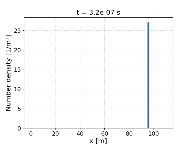
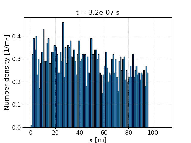
The incident particles in the Electron_bunch species initially have a number density of 100/m³. At the end of the simulation, they still travel in a bunch, but the density has dropped since they are destroyed upon triggering test_process_emission.

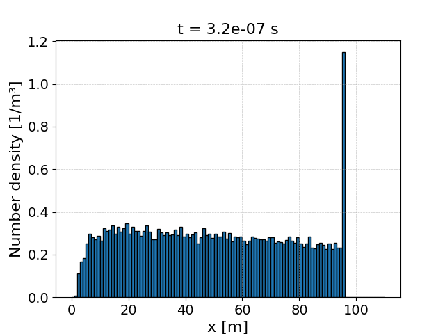
Each time a macro-particle from the Electron_bunch species is destroyed, a new identical macro-electron is created in the Moving_new_electrons species. This should keep the number of real-electrons in the bunch constant. The final density of the Moving_new_electrons species is shown below, and when summing this with the final Electron_bunch density, we recover the original 100/m³.

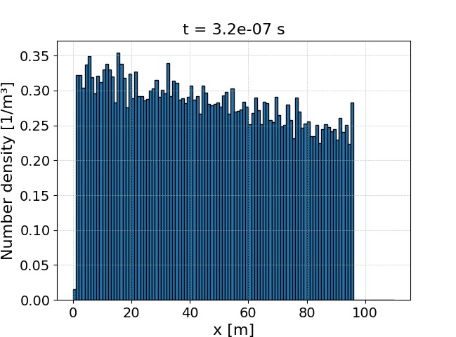
Finally, at the site of each emission, a stationary macro-electron is created. When looking at the density of Still_new_electrons, we can observe the expected exponential decay pattern from the constant-rate test_process_emission process.

Example 2.1

This example has the same setup as Example 2.0, but one of the secondary species is missing from the physics_package block:

begin:physics_package
   process = test_process_emission
   incident = Electron_bunch
   secondary1 = Moving_new_electrons
end:physics_package

Currently, when a secondary species is missing, the code will create a new species for this secondary, using a name found from the overriden function get_new_spec_names() in each derived physics package.

In FORTRAN, the ionisation subroutines are able to create new species, so it is important that the C++ physics packages can too. However, the C++ implementation is currently quite basic, and will be modified when real physics packages are added later. For example, in bremsstrahlung, the code could look for any pre-existing photon species before creating a new species. At the moment, any missing species will be assumed to be an electron.

To demonstrate that a stationary-electron species was created in this case, we plot its final number density here:

Example 2.2

In the code, it is possible to boost the number of created secondary macro-particles, while conserving the number of real particles. This is done by increasing the rate at which the process is triggered, but only producing secondaries with a scaled-down weight. Additionally, any effects applied to the incident macro-particle will no longer activate each time the process triggers, and will instead be done with a probability related to the scaling factor. This ensures incident particles behave as they did without the secondary boost.

This feature allows us to obtain better secondary spectra by performing more samples, which is especially useful in rarer processes. To increase the number of created macro-particles by a factor of 5, we may run

begin:physics_package
   process = test_process_emission
   incident = Electron_bunch
   secondary1 = Moving_new_electrons
   secondary2 = Still_new_electrons
   boost_secondaries = 5
end:physics_package

Let us compare the output to Example 2.0, which describes a physically identical system without secondary boosting. The number of surviving incident particles is still the same:

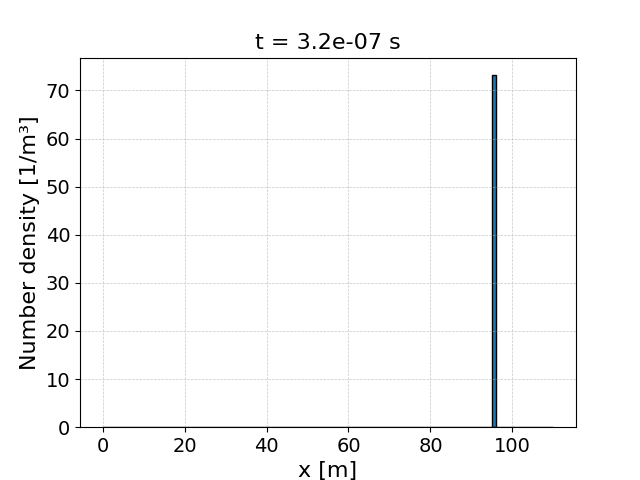
When we look at the secondary macro-electrons in the stationary species, which shows where test_process_emission was triggered, we see the same exponential decay as before. However, since more macro-particles were sampled in this example, the distribution is seen to be less noisy.

Example 2.3

Similarly to Example 2.2, the rate of secondary macro-particle creation can also be reduced, while conserving the number of real secondary particles. This is useful in cases where the rate of secondary production is too high, and memory starts to suffer from too many macro-particles being created.

The process trigger rate is fixed, and incident macro-particles are always affected by the process, but secondary macro-particles are only created with a probability related to the boost number. If secondaries are created, their weights are increased to conserve the number of real particles produced.

This secondary-reduction feature can be used by boosting the secondaries with a number less than 1:

begin:physics_package
   process = test_process_emission
   incident = Electron_bunch
   secondary1 = Moving_new_electrons
   secondary2 = Still_new_electrons
   boost_secondaries = 0.1
end:physics_package

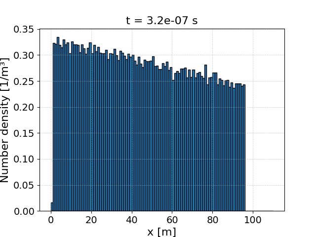
When looking at the density of the stationary secondary species, which shows where test_process_emission was triggered, we see the same exponential decay behaviour as in Example 2.0 and 2.2. The data is noisier in this current example as fewer macro-particles have been created:

Example 2.4

When new particles are created, its important that any MPI-aware permanent particle variables are correctly initialised. To show that this is the case, we have applied the test_process_single package to our newly created Moving_new_electrons species:

begin:physics_package
   process = test_process_emission
   incident = Electron_bunch
   secondary1 = Moving_new_electrons
   secondary2 = Still_new_electrons
end:physics_package

begin:physics_package
   process = test_process_single
   incident = Moving_new_electrons
end:physics_package

Not only will this test if the physics package manager can handle multiple processes, but it will also test if the optical-depth for the test_process_single package is correctly initialised for the Moving_new_electrons species. This is the same package as featured in Example 1, which has a constant rate of triggering, and sets the momentum of triggered macro-electrons to 0.

In previous examples, the Moving_new_electrons species would travel with the incident Electron_bunch species, but now test_process_single would stop them. The final density of this species is shown here:

We see that while some of the electrons are travelling with the incident Electron_bunch species, and almost reaching 100m, many others have stopped before then due to triggering test_process_single. Any secondary electrons still travelling with the incident bunch were likely created recently, and haven’t had enough time to stop under a test_process_single trigger yet.

Given that we have a mix of stationary and moving particles in the Moving_new_electrons species shows that the optical-depth was correctly set for each new electron - otherwise they would all trigger test_process_single immediately, and there wouldn’t be a density spike at the incident bunch location.