
Bethe-Heitler e-e+#
Bethe-Heitler pair production refers to a process where an incident photon decays to a lepton pair in the presence of the Coulomb fields surrounding an ion or atom. On this page, we will consider the decay to an electron/positron pair.
Cross sections#
Cross sections for the Bethe-Heitler conversion of photons to electron/positron pairs are tabulated in Table 6 of “Hubbell (1980) J. Phys. Chem. Reference Data, 9(4), 1023-1148”, which is currently available through NIST: https://srd.nist.gov/JPCRD/jpcrd169.pdf.
A method to sample cross-sections from this data has been provided by the Geant4 Physics Reference Manual, which involves the following fit functions:
\(x = \ln\left(\frac{E_\gamma}{m_e c^2}\right)\)
\(f_1(x) = 878.42 - 1962.5x + 1294.9x^2 - 200.28x^3 + 12.575x^4 - 0.28333 x^5\)
\(f_2(x) = -10.342 + 17.692x - 8.2381x^2 + 1.3063x^3 -0.090815x^4 + 0.0023586x^5\)
\(f_3(x) = -452.63 + 1116.1x - 867.49x^2 + 217.73x^3 -20.467x^4 + 0.65372x^5\)
where \(E_\gamma\) is the photon energy, and \(m_e c^2\) is the electron rest mass energy. These functions are used to obtain a cross-section, \(\sigma\) via:
\(\sigma = (Z + 1)(f_1(x)Z + f_2(x)Z^2 + f_3(x)) \times 10^{-34} \text{ m}^2\)
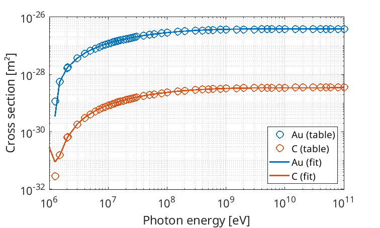
for a target with atomic number \(Z\). This fit includes contributions from both the “nuclear field” and the “electron field” columns of the Hubbell Table 6 data. Good agreement can be seen between the fit and the Hubbell tabulated values in different materials:
Pair particle energies#
The energies of the created electron and positron can be sampled using the differential cross-section of Bethe-Heitler pair production, which is given in equation (3D-1003) of “Motz (1969) Reviews of Modern Physics, 41(4), 581”. This function varies as:
\(f(\epsilon) \propto (\epsilon^2 + (1 - \epsilon)^2)(\Phi_1(G) - \frac{4}{3}\ln(Z)) + \frac{2}{3}\epsilon(1-\epsilon)(\Phi_2(G) - \frac{4}{3}\ln(Z))\)
where \(\epsilon = E_e / E_\gamma\), \(E_\gamma\) is the incident photon energy, and \(E_e\) is the total energy of whichever particle in the created pair has the lowest energy. This functional form is valid for a screened point nucleus in extreme relativistic cases, and includes the screening functions \(\Phi_1(G)\) and \(\Phi_2(G)\), which are approximated by Butcher and Messel using:
\(G = \frac{136 m_e c^2}{E_\gamma\epsilon(1-\epsilon) Z^{1/3}}\)
For \(G\leq 1\), the screening terms may be written:
\(\Phi_1(G) = 20.868 - 3.242G + 0.625G^2\)
\(\Phi_2(G) = 20.209 - 1.930G + 0.086G^2\)
while for \(G > 1\):
\(\Phi_1(G) = 21.12 - 4.184 \ln(G + 0.952)\)
\(\Phi_2(G) = \Phi_1(G)\)
In order to sample from this function, tables are constructed during the physics-package setup. A subset of values for the \(Z=79\) gold table is shown below:
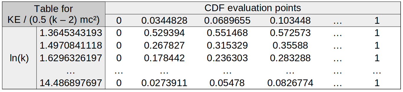
where \(k = E_\gamma / m_ec^2\), and \(KE\) refers to the kinetic energy of the pair-particle with the lowest energy. The table quotes values of the kinetic energy for the low-energy pair particle, evaluated at different sample points along the CDF distribution. These kinetic energies are normalised to the maximum kinetic energy which can be achieved by the low-energy particle, which occurs when both particles take half the photon energy each.
This table is calculated by evaluating \(f(\epsilon)\) at different \(\epsilon\) for a given \(k\), and then normalising the distribution to get a probability density function. The CDF is then deduced from the PDF integral at many different points, providing a list of CDF values for the different kinetic energies. This list is then interpolated to the CDF sample points, which are equally spaced to allow fast table look-up.
Whether the electron or positron is the lower-energy particle is decided randomly, with an equal chance for each particle to have the lower energy.
Angular distribution#
The EPOC++ Bethe-Heitler model for e-/e+ pair production uses the Geant4 model for the angular distribution function \(f(\gamma\theta)\):
\(f(\gamma\theta) = \frac{a^2\gamma\theta}{4}\left( e^{-a\gamma\theta} + 27e^{-3a\gamma\theta} \right)\)
where \(\theta\) is the angle between the momentum of a pair particle and the incident photon, \(\gamma\) is the pair-particle Lorentz factor, and the fit parameter \(a = 0.625\). Here, \(\theta\) will only be accepted between 0 and \(\pi\). The value of \(\gamma\theta\) is sampled once, and applied to both pair-particles, which gives different \(\theta\) values to particles with different energies.
The azimuthal angle \(\phi\) for one particle is sampled randomly between 0 and \(2\pi\), and the other particle is rotated to \(\phi + \pi\).
The sampling method is similar to that performed for bremsstrahlung:
Generate 3 uniformly distributed random numbers between 0 and 1: \(r_1\), \(r_2\), \(r_3\)
If \(r_1 < 0.25\), \(b = 0.625\), otherwise \(b = 1.875\)
\(\theta_\pm = - \ln(r_2 r_3) / \gamma_\pm b\)
Example: Bethe-Heitler#
In this example, \(5 \times 10 ^5\) photons are initialised in the first 5 cells
on the x_min boundary, and are each set to an energy of 100 MeV. These photons
propagate through 2 cm of solid-density Au, and the Bethe-Heitler \(e^-e^+\)
process is switched on. Macro-particles created for the Electron and
Positron species are set to be immobile, such that their positions at the end
of the simulation describe where they were created.
From the Hubbell tables, 100 MeV photons in gold have a cross-section of \(2.94 \times 10^{-27}\) m². For a gold target with density \(6.0 \times 10^{28}\) /m³, this corresponds to a pair-production rate of around \(5.3 \times 10^{10}\) /s. Since the photons have a constant rate of decay, we can produce a theoretical exponential to estimate how many survive to a given depth before undergoing pair production. This can be used to estimate the number density of immobile pairs as a function of depth, which has been modelled with EPOC++, and compared to theory:

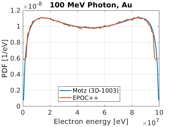
The energy spectrum of produced electrons was also calculated, and normalised to show a probability density function. This was then compared to the PDF expected from Eq. (3D-1003) in Motz, and it was found that the energy distribution could be accurately reproduced:
These plots were produced using the input deck below:
begin:control
  nx = 256
  x_min = 0
  x_max = 0.02
  t_end = 67e-12
  verbose = 2
  stdout_frequency = 10
end:control

begin:boundaries
  bc_x_min = open
  bc_x_max = open
end:boundaries

begin:physics_package
  process = bethe_heitler_ee
  incident = Photon_bunch
  background = Gold
  electron_species = Electron
  positron_species = Positron
end:physics_package

begin:species
  name = Photon_bunch
  drift_x = 5.341e-20
  rho = 1.0e5 * nx / (x_max - x_min)
  rho = if (x lt 5*dx, density(Photon_bunch), 0)
  npart = 2048000
  identify:photon
end:species

begin:species
  name = Gold
  atomic_number = 79
  charge = 0
  mass = 359109
  rho = 6.0e28
  npart_per_cell = 2000
  immobile = T
end:species

begin:species
  name = Electron
  immobile = T
  identify:electron
end:species

begin:species
  name = Positron
  immobile = T
  identify:positron
end:species

begin:output
  name = rst
  nstep_snapshot = 10
  rolling_restart = F
  dump_first = T
end:output