Field ionisation

Field ionisation describes ionisation due to the interaction of atoms/ions with an external electric field. The field ionisation package in EPOCH calculates ionisation rates following the method described in the thesis of Lawrence-Douglas (2013): “Ionisation effects for laser-plasma interactions by particle-in-cell code”. This approach combines rates from multiphoton absorption, electron tunnelling, and a classical barrier suppression model based on orbital electron geometry. The particular model chosen depends on the magnitude of the background electric field, with different processes used in different regimes. An interpolation method has been taken from the Lawrence-Douglas thesis, which ensures the ionisation rate rises smoothly in most cases.

In addition to the Lawrence-Douglas method, an alternative classical ionisation rate has been provided, which uses different approximations to the one present in the thesis. The intention of this extra model is to describe ionisation in systems where the external electric field is considerably stronger than the binding field, as it is unclear how well the assumptions of the classical method used by Lawrence-Douglas perform in these systems.

The ionisation energy and quantum numbers of the outermost bound electrons in the ion are read from file. The details of this may be found in the collisional ionisation documentation. The field ionisation package does not use the binding energy, mean bound kinetic energy, or occupancy number data.

Multiphoton ionisation

Multiphoton ionisation is described in Section 2.2.1 of the Lawrence-Douglas thesis, using theory which may be found in the Delone and Krainov (1994) textbook “Multiphoton processes in atoms” (first edition). Multiphoton theory requires us to determine the number of photons required to ionise the ion, \(K\). Here, \(K\) is the smallest integer which satisfies \(K\hbar \omega \leq I\), where \(I\) is the ionisation energy of the current ion, and \(\omega\) is the angular frequency of the laser. Cells in EPOCH are described with a single field value, which is insufficient to deduce the laser frequency on its own - hence, this package requires a user-provided angular frequency to work with.

The ionisation rate \(\lambda\) is given by Delone & Krainov Eq. (1.2), or equivalently, Lawrence-Douglas Eq. (2.7):

\(\lambda = \hat{\sigma}^{(K)} \left( \frac{c' E'^2}{8 \pi \omega'} \right)^K \left( \frac{\hbar}{r_0^2 m_e} \right)\)

which has been converted to SI units here. The electric field strength \(E\) and the laser angular frequency \(\omega\) have been given in atomic units:

\(E' = E \left(\frac{r_0^3 m_e e }{\hbar^2}\right)\)

\(\omega' = \omega \left( \frac{r_0^2 m_e }{\hbar} \right)\)

where \(r_0\) is the Bohr radius, with electron mass and charge \(m_e\) and \(-e\) respectively. The speed of light in atomic units is written

\(c' = c \left( \frac{r_0 m_e}{\hbar} \right)\).

The generalised multi-photon cross section is quoted in Eq. (5.29) of Delone (1994) as:

\(\hat{\sigma}^{(K)} = T_K E'^{2K-2} \frac{1}{c'(K!)^2 n^5\omega'^{(10K-1)/3}}\)

where \(n\) refers to the principal quantum number of the outermost bound electron. Delone (1994) also provides an expression for the factor \(T_K\), for linearly polarised lasers in their Eq. (5.30):

\(T_K = 4.80 (1.30)^{2K} \frac{1}{(2K+1)\sqrt{K}}\)

These combine to give Eq. (2.8) in the Lawrence-Douglas thesis, with one typo in the Lawrence-Douglas version (\(2K+1\) is written as \(2K-1\)). An expression for circular polarisation is provided in Delone (1994) Eq. (5.31), but is not implemented in EPOCH. This involves replacing the factor \(4.80 (1.30)^{2K}\) with \(7.52 (1.41)^{2K}\) in the \(T_K\) expression.

As discussed in Ilkov (1992) J. Phys. B: At. Mol. Opt. Phys. 25 4005, the multiphoton ionisation rates are most appropriate in regimes with \(\gamma_k \ll 1\), for Keldysh parameter \(\gamma_k\):

\(\gamma_k = \frac{\omega'}{E'}\sqrt{2 I'}\)

where \(I'\) is the ionisation energy in atomic units:

\(I' = I \left(\frac{r_0^2 m_e}{\hbar^2}\right)\)

Tunnelling ionisation

In tunnelling ionisation, the external electric field-strength approaches the fields binding the electron to the ion. This lowers the total field felt by the bound electron, allowing it to ionise by tunnelling away from the ion. The process was described by Ammosov, Delone, Krainov (1986), Sov. Phys. JETP 64(6) (not the SPIE version), and the tunnelling rate is sometimes referred to as the ADK rate after these authors. This theory is summarised in Section 2.2.2 of Lawrence-Douglas (2013).

Combining Eq. (1), (2) and (19) of Ammosov (1986) yields the tunnelling rate quoted in Eq. (2.9) of Lawrence-Douglas (2013), and after converting to SI units, this reads:

\(\lambda = \frac{2^{2n^*}I'}{n^* \Gamma(n^*+l^*+1)\Gamma(n^*-l^*)}\left(\frac{3E'}{\pi E_0'}\right)^{1/2} \frac{(2l+1)(l+|m|)!}{2^{|m|}(|m|)!(l-|m|)!}\)

\(\times \left(\frac{2E_0'}{E'}\right)^{2n^*-|m|-1}\exp\left(-\frac{2E_0'}{3E'}\right)\left(\frac{\hbar}{r_0^2 m_e}\right)\)

where \(E_0' = (2I')^{3/2}\), \(n^*=Q/\sqrt{2I'}\), \(l^*=n_0^*-1\). Here, \(Q\) is the charge-state of the ion after ionisation, \(n^*\) and \(n_0^*\) are the effective principal quantum numbers of the current state and ground state respectively, and \(nlm\) are the quantum numbers of the outermost bound electron. Here we have corrected a typo in Lawrence-Douglas (2013) Eq. (2.9), where the term to the power of \(2n^*-|m|-1\) was missing a factor of 2.

Lawrence-Douglas goes further, assuming the ion is in its ground-state \(n^* = n_0^*\). Additionally, while the outermost \(n\) and \(l\) values may be read from file, EPOCH does not track the \(m\) of the outermost electron. Instead, we may average the rate over all \(m\) values. Firstly, let rewrite the rate as:

\(\lambda_m = \sqrt{\frac{6}{\pi}}\left(\frac{\hbar}{r_0^2 m_e}\right) \frac{2^{2n^*} I'}{n^* \Gamma(2n^*)} \left(\frac{2 E_0'}{E'}\right)^{(4n^*-3)/2}\exp\left(-\frac{2E_0'}{3E'}\right)\)

\(\times\left(\frac{(2l+1)(l+|m|)!}{2^{|m|}(|m|)!(l-|m|)!} \left(\frac{2E_0'}{E'}\right)^{-|m|} \right)\)

where the line-break has been chosen to separate out terms which depend on \(m\).

EPOCH averages over all possible \(m\) for the tunnelling rate, such that

\(\langle \lambda \rangle = \frac{1}{2l + 1}\sum_{m=-l}^{m=l} \lambda_m\)

which returns the expression given by Lawrence-Douglas (2013) Eq. (2.18), which in SI units reads:

\(\langle\lambda\rangle = \sqrt{\frac{6}{\pi}}\left(\frac{\hbar}{r_0^2 m_e}\right) \frac{2^{2n^*} I'}{n^* \Gamma(2n^*)} \left(\frac{2 E_0'}{E'}\right)^{(4n^*-3)/2}\exp\left(-\frac{2E_0'}{3E'}\right)\)

\(\times \left(\sqrt{\frac{16E_0'}{\pi E'}}\exp\left(\frac{2E_0'}{E'}\right) K_{l+1/2}\left(\frac{2 E_0'}{E'}\right) - 1\right)\)

where \(K_{l+1/2}\left(2 E_0'/E'\right)\) is a modified Bessel function of the second kind. Here we have used the identity:

\(K_{l+1/2}(x) = \sqrt{\frac{\pi}{2x}}e^{-x} \sum_{m=0}^{m=l} \frac{(l+m)!}{2^m m! (l-m)!}x^{-m}\)

for positive integer values of \(l\).

As shown in Ilkov (1992) Eq. (9), these tunnelling ionisation rates are most accurate between field values of:

\(2 \omega' \sqrt{2 I'} < E' < \frac{I'^2}{4 Q}\)

where the lower limit corresponds to a Keldysh parameter of 0.5, and the upper limit describes the classical binding electric field strength.

Barrier-suppression ionisation (classical)

When the external field becomes greater than the classical binding field, bound electrons are able to freely leave the ion. An ionisation rate for this regime has been estimated in a paper by Posthumus et al, which can be found starting on pg. 298 of the 1996 textbook “Proceedings of the 7th conference on multiphoton processes held in Garmisch-Partenkirchen, Germany” (currently available on the online “Open Library”). This paper is summarised in Section 2.2.3 of Lawrence-Douglas (2013).

In the classical ionisation theory, bound electrons are assumed to orbit the nucleus with some characteristic period, within a binding equipotential sphere. An external electric field will deform that equipotential surface, and once the external field exceeds the binding field, a hole opens in the surface which allows electrons to escape. The ionisation rate is taken to be the fractional solid-angle size of this equipotential hole compared to the total surface, divided by the period of electron orbit. This can be thought of as a probability of being somewhere where the electron can escape, divided by a characteristic time-scale for bound electron exploration.

On pg. 299 of the proceedings book, Posthumus writes the classical orbital period as:

\(T_0 = \frac{\pi Q}{\sqrt{2} |I'|^{3/2}}\)

An ionisation rate is given on pg. 300, which matches Eq. (2.10) in Lawrence-Douglas (2013). In SI units, this equation reads:

\(\lambda = \frac{\left(2I'\right)^{3/2}\left(1 - \frac{I'^2}{4QE'}\right)}{4\pi Q}\left(\frac{\hbar}{r_0^2 m_e}\right) + \lambda_{ADK}\left(E'_{b}\right)\)

where \(\lambda_{ADK}\left(E'_{b}\right)\) refers to the tunnelling ionisation rate evaluated at the classical binding field \(E'_{b}\), which in atomic units reads:

\(E'_{b} = \frac{I'}{4Q}\)

which is equivalent to the term \(E_c\) in Lawrence-Douglas (2013) Eq. (2.10).

Classical ionisation (strong-field)

In the Posthumus (1996) barrier-suppression ionisation theory, we assume an electron orbits around an ion until it encounters a hole in an equipotential surface, deformed by an external field. It is unclear how well this theory describes ionisation in electric fields significantly stronger than the binding field. Instead, we will also provide an optional model for a simple, classical, high-field ionisation rate.

In SI units, the classical binding field from the upper limit of Ilkov (1992) Eq. (9) reads

\(E_{b} = \frac{I'}{4Q} \left(\frac{\hbar^2}{r_0^3 m_e e}\right)\)

In this simple model, we will assume the net electric field is \(E-E_b\), for external field \(E\). Let us calculate the time taken, \(t_0\), for an electron to accelerate from rest to having a kinetic energy equal to the ionisation energy in this field. The ionisation rate will be assumed to be \(1/t_0\), such that

\(\lambda = \frac{ec(E-E_b)}{\sqrt{(I+m_ec^2)^2 - m_e^2 c^4}}\)

This model was devised while writing this documentation, and there is no associated reference. We include this as an alternative to the Posthumus (1996) method, for people who wish to test the sensitivity of their results against their classical approximations.

Combined ionisation rate

Multiphoton ionisation, tunnelling ionisation, and the classical models for barrier-suppression ionisation all provide rates (\(\lambda_\text{multi}, \lambda_\text{ADK}, \lambda_\text{BSI}\)) which are valid for different background electric field strengths. These models are less accurate in describing the transition regions: from multiphoton to tunnelling, or from tunnelling to barrier-suppression. Let us plot all these ionisation rates as a function of laser intensity \(I_0\), using \(I_0 = \epsilon_0 c E^2 / 2\) to get the corresponding electric field strength. The figure below was created for the \(\text{H}\rightarrow \text{H}^+\) transition, with a 2 \(\mu\text{m}\) laser.

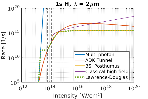
Three vertical dashed lines have been provided here. Moving from left to right, we have:

• \(E_1\): Field-strength where \(E' = 2\omega'\sqrt{2I'}\), lower limit for the tunnelling regime, from Ilkov (1992) Eq. (9).

• \(E_2\): Field-strength where \(E' = I'^2/4Q\), classical binding field and upper limit of the tunnelling regime, from Ilkov (1992) Eq. (9).

• \(E_3\): Field corresponding to the maximum rate for the tunnelling model, where \(d\lambda_{ADK}/dE=0\).

For \(E_3\), EPOCH calculates \(\lambda_{ADK}\) for increasing \(E\), and returns the first \(E\) which causes the rate to drop. If this method fails, an approximation is used where the stationary point is calculated using only the \(m=0\) rate:

\(E_3 = \frac{2 (2I')^{3/2}}{3(2n^*-1.5)} \left(\frac{\hbar^2}{r_0^3 m_e e}\right)\)

For electric fields much smaller than \(E_1\), the multiphoton approach is valid. The tunnelling regime exists between \(E_1\) and \(E_2\), and barrier suppression techniques are valid for \(E>E_2\). However, these models do a poor job describing the transition regions.

In Lawrence-Douglas (2013) Section 2.3.2, an interpolation method is proposed to address this uncertainty. The procedure is summarised in their Eq. (2.21), and it is designed to make the ionisation rate increase with the field strength.

• \(E < E_1\): Use multiphoton rates until they become too large. Let \(\lambda = \min(\lambda_\text{multi}(E), \lambda_\text{ADK}(E_1))\)

• \(E_1 < E < E_2\): Tunnelling regime, \(\lambda = \lambda_\text{ADK}(E)\)

• \(E_2 < E < E_3\): To avoid a sharp transition between tunnelling and barrier-suppression, use whichever rate is lowest, \(\lambda = \min(\lambda_\text{ADK}(E), \lambda_\text{BSI}(E))\)

• \(E > E_3\): Tunnelling rates start to fall. Switch to barrier suppression if we haven’t already, \(\lambda = \lambda_\text{BSI}(E)\).

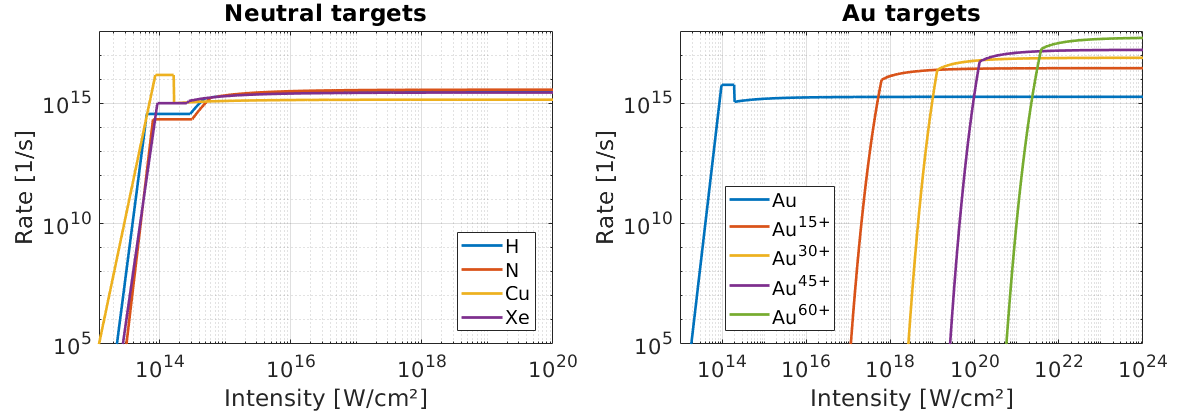
This interpolation method does not guarantee that the rates increase with electric field strength, but they do in most cases. By default, the Lawrence-Douglas (2013) method uses the Posthumus (1996) barrier-suppression model, but this may be swapped out for the classical high-field model if specified in the input deck. Ionisation rates using the default model have been given below for various different targets, under illumination from a laser of wavelength 1 \(\mu\text{m}\).

Field energy loss

During a field ionisation event, energy is lost from the laser to ionise a bound electron. In multiphoton ionisation, each real ionised electron absorbs energy \(\Delta \epsilon = K\hbar\omega\), while electrons undergoing tunnelling or barrier-suppression ionisation absorb energy \(\Delta \epsilon = I\). For an ionised macro-ion of weight \(W_i\), the electric-field energy-density should change as

\(\Delta U = \frac{W_i \Delta\epsilon}{V}\)

where \(V\) is the cell volume. Since the energy density of an electric field is

\(U = \frac{1}{2}\epsilon_0 E^2\)

we have

\(\frac{\partial U}{\partial t} = \epsilon_0 \vec{E} \cdot \frac{\partial \vec{E}}{\partial t}\)

From the Ampere-Maxwell law, ignoring \(B\) fields, we have:

\(\frac{\partial \vec{E}}{\partial t} = -\frac{1}{\epsilon_0} \vec{J}\)

Hence, adding a current density will change the electric field strength, and a changing electric field strength leads to a change in the electric-field energy-density. In order to force the laser to lose energy, we may simply add a fake current-density to the grid. If we assume this current is parallel to the electric field, we may combine the above equations to obtain an expression for the correction current density

\(\vec{J} = \frac{W_i \Delta\epsilon}{VE^2\Delta t}\vec{E}\)

which is equivalent to Lawrence-Douglas (2013) Eq. (2.22), where we have included a missing \(V\) factor.

Ionisation kinematics

When a macro-particle with mass \(m_0\) and momentum \(p_0\) undergoes ionisation, we create a macro-ion of mass \(m_0-m_e\), and a macro-electron of mass \(m_e\). In tunnelling and barrier-suppression ionisation, we assume the electron absorbs only enough laser energy to ionise. The momentum of the initial particle is then split between the macro-ion and macro-electron, according to the mass-fraction. The electron momentum, \(p_e\), and ion momentum \(p_i\) take the form:

\(p_e = \frac{m_e}{m_0} p_0\)

\(p_i = \left(1 - \frac{m_e}{m_0}\right) p_0\)

However, in multiphoton ionisation, the absorbed energy \(K\hbar\omega\) may be greater than the ionisation energy \(I\). In this case, the excess energy is assumed to take the form of electron kinetic energy. Assuming this excess energy is always small enough to be non-relativistic, we therefore set

\(p_e = \frac{m_e}{m_0} p_0 + \sqrt{2 m_e (K\hbar\omega - I)}\)

for electrons ionised by the multiphoton process.

Example: Multiphoton

Consider the ionisation of \(\text{N}\rightarrow\text{N}^+\), under the influence of a uniform electric field. All particles are kept immobile, so any current density on the grid can only be created by the field ionisation process. The nitrogen density is kept sufficiently low that any energy loss by the background \(E\) field is negligible. We will set-up the field ionisation package to treat the \(E\) field as being a laser of wavelength 1 \(\mu\text{m}\).

In this example, we will set \(E_y = 2.32\times10^{10} \text{ V/m}\), which puts us in the multi-photon ionisation regime. Since the \(E\) field is roughly uniform and constant, the field ionisation rate will be fixed at around \(\lambda = 2.17\times10^{13}\text{ s}^{-1}\) over the full simulation. This allows us to estimate the N number density as a function of time, which is shown below

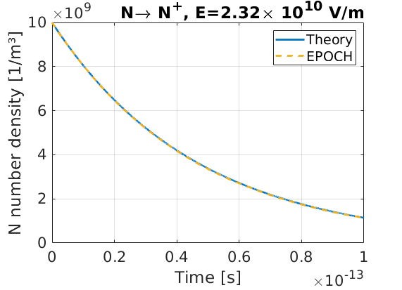
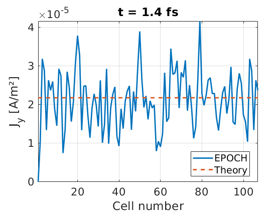
Here we see good agreement between the expected ionisation rate, and the observed. Let us also check the current density on the grid, at an early time. Near the start of the simulation, the expected change in number density is:

\(\Delta n_i \approx n_i(t=0) \left( 1 - e^{-\lambda \Delta t}\right)\)

which, for small \(\lambda\Delta t\), we have

\(\Delta n_i \approx n_i(t=0)\lambda \Delta t\)

Using Lawrence-Douglas (2013) Eq. (2.22), we can estimate the corrective current density at early times to be

\(J_y \approx \frac{n_i(t=0) \lambda I}{E_y}\)

Plotting the current density at early times shows that we do generate the expected \(J_y\)

begin:control
  nx = 100
  x_min = 0
  x_max = 4.5e-6
  t_end = 100.0e-15
  verbose = 2
  stdout_frequency = 1
end:control

begin:boundaries
  bc_x_min = periodic
  bc_x_max = periodic
end:boundaries

begin:fields
  ey = 2.32e10
end:fields

begin:physics_package
  process = field_ionisation
  incident = Nitrogen
  ionise_to_species = Nitrogen1
  ejected_electron = Ejected_electron
  laser_omega = 2 * pi * c / 1.0e-6 
end:physics_package

begin:species
  name = Nitrogen
  atomic_number = 7
  charge = 0
  mass = 25532.7
  rho = 1.0e10
  npart_per_cell = 1000
  immobile = T
end:species

begin:species
  name = Nitrogen1
  atomic_number = 7
  charge = 1
  mass = 25532.7 - 1
  immobile = T
end:species

begin:species
  name = Ejected_electron
  immobile = T
  identify:electron
end:species

begin:output
  name = rst
  nstep_snapshot = 10
  rolling_restart = F
  dump_first = T
end:output

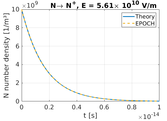
Example: Tunnelling

This example uses the same setup as the multiphoton ionisation example, but here we set the background electric field to \(E_y = 5.61\times10^{10} \text{ V/m}\). This puts us in the tunnelling regime, where we would expect an ionisation rate of \(\lambda = 5.95\times10^{14}\text{ s}^{-1}\). A plot of nitrogen number density as a function of time shows that the rate has been correctly calculated in EPOCH.

begin:control
  nx = 1000
  x_min = 0
  x_max = 4.5e-6
  t_end = 10.0e-15
  verbose = 2
  stdout_frequency = 1
end:control

begin:boundaries
  bc_x_min = periodic
  bc_x_max = periodic
end:boundaries

begin:fields
  ey = 5.61e10
end:fields

begin:physics_package
  process = field_ionisation
  incident = Nitrogen
  ionise_to_species = Nitrogen1
  ejected_electron = Ejected_electron
  laser_omega = 2 * pi * c / 1.0e-6 
end:physics_package

begin:species
  name = Nitrogen
  atomic_number = 7
  charge = 0
  mass = 25532.7
  rho = 1.0e10
  npart_per_cell = 100
  immobile = T
end:species

begin:species
  name = Nitrogen1
  atomic_number = 7
  charge = 1
  mass = 25532.7 - 1
  immobile = T
end:species

begin:species
  name = Ejected_electron
  immobile = T
  identify:electron
end:species

begin:output
  name = rst
  nstep_snapshot = 10
  rolling_restart = F
  dump_first = T
end:output

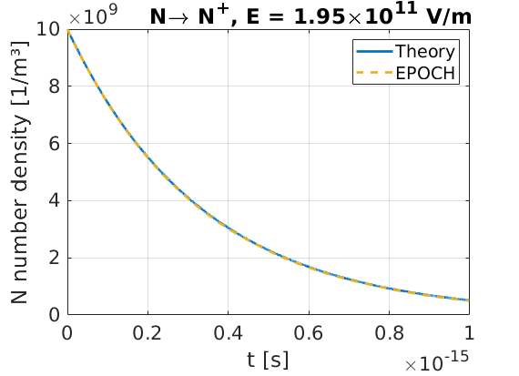
Example: Barrier-suppression

This example uses the same setup as the multiphoton ionisation example, but here we set the background electric field to \(E_y = 1.95\times10^{11} \text{ V/m}\). This puts us in the barrier-suppression regime, where we would expect an ionisation rate of \(\lambda = 2.97\times10^{15}\text{ s}^{-1}\). A plot of nitrogen number density as a function of time shows that the rate has been correctly calculated in EPOCH.

begin:control
  nx = 10000
  x_min = 0
  x_max = 4.5e-6
  t_end = 1.0e-15
  verbose = 2
  stdout_frequency = 1
end:control

begin:boundaries
  bc_x_min = periodic
  bc_x_max = periodic
end:boundaries

begin:fields
  ey = 1.95e11
end:fields

begin:physics_package
  process = field_ionisation
  incident = Nitrogen
  ionise_to_species = Nitrogen1
  ejected_electron = Ejected_electron
  laser_omega = 2 * pi * c / 1.0e-6 
end:physics_package

begin:species
  name = Nitrogen
  atomic_number = 7
  charge = 0
  mass = 25532.7
  rho = 1.0e10
  npart_per_cell = 10
  immobile = T
end:species

begin:species
  name = Nitrogen1
  atomic_number = 7
  charge = 1
  mass = 25532.7 - 1
  immobile = T
end:species

begin:species
  name = Ejected_electron
  immobile = T
  identify:electron
end:species

begin:output
  name = rst
  nstep_snapshot = 10
  rolling_restart = F
  dump_first = T
end:output

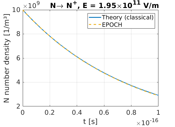
Example: Classical model

This example uses the same setup as the multiphoton ionisation example, but here we set the background electric field to \(E_y = 1.95\times10^{11} \text{ V/m}\). This puts us in the barrier-suppression regime, but unlike the previous example, we have switched off the default Posthumus (1996) rate. Instead, we will use the classical strong-field ionisation model, which gives a rate of \(\lambda = 1.23\times10^{16}\text{ s}^{-1}\). A plot of nitrogen number density as a function of time shows that the rate has been correctly calculated in EPOCH.

begin:control
  nx = 100000
  x_min = 0
  x_max = 4.5e-6
  t_end = 0.1e-15
  verbose = 2
  stdout_frequency = 1
end:control

begin:boundaries
  bc_x_min = periodic
  bc_x_max = periodic
end:boundaries

begin:fields
  ey = 1.95e11
end:fields

begin:physics_package
  process = field_ionisation
  incident = Nitrogen
  ionise_to_species = Nitrogen1
  ejected_electron = Ejected_electron
  laser_omega = 2 * pi * c / 1.0e-6
  use_multiphoton = T
  use_tunnelling = T
  use_barrier_suppression = F
  use_classical_rate = T
end:physics_package

begin:species
  name = Nitrogen
  atomic_number = 7
  charge = 0
  mass = 25532.7
  rho = 1.0e10
  npart_per_cell = 1
  immobile = T
end:species

begin:species
  name = Nitrogen1
  atomic_number = 7
  charge = 1
  mass = 25532.7 - 1
  immobile = T
end:species

begin:species
  name = Ejected_electron
  immobile = T
  identify:electron
end:species

begin:output
  name = rst
  nstep_snapshot = 10
  rolling_restart = F
  dump_first = T
end:output