
Nuclear trident#
In the nuclear-trident process, an incident electron creates an \(e^-e^+\) pair when interacting with the Coulomb field of a target nucleus. The theory for this interaction is given in “Bhabha (1935) Proc. Royal Soc. London, Series A, 152(877), 559-586”. Quantities are sampled from theory using fits descibed by “Martinez (2019) Physics of Plasmas, 26(10)”, and also “Gryaznykh (1998) J. of Exp. and Theoretical Phys. Lett., 67, 257-262”.
Cross sections#
In Eq. (3) of Gryaznykh (1998), a model for the cross-section is presented which transitions between theoretical cross-sections at the low and high incident energy limits. This fit is re-arranged by Martinez (2019) in Eq. (26) to give:
\(\sigma = Z^2 \ln^3(\frac{\gamma_1 + 4.50}{6.89})\times 5.22\times 10^{-34} \text{ m}^2\)
where \(Z\) is the atomic number of the target, and \(\gamma_1\) is the Lorentz factor for the incident electron.
Pair particle energies#
The energies of the created electron and positron are sampled through a two-step process, using tables calculated at the start of the simulation. In the first sample, a “pair energy” is obtained using the incident particle energy.
The incident particle energy, \(E_1\) is sampled with a uniform logarithmic spacing between \(3m_ec^2\) (incident and pair particles finish at rest) and 10 GeV. For each \(E_1\), possible pair energies are sampled with uniform linear spacing from \(2 m_e c^2\) to \(E_1 - m_e c^2\). The differential cross-section for each combination of incident and pair energies is calculated using a procedure outlined by Martinez (2019) in section IID. This begins by calculating the auxilliary functions in Eq. (29):
\( x = \frac{1}{\gamma_1} \)
\( C = 4 \frac{x^2}{1- x^2} \ln\left(\frac{1}{x^2}\right) - \frac{4}{3} x^2 + \frac{1}{6}x^4\)
\(C_z = 3 \frac{x^2}{1 - x^2} \left( 1 - \frac{x^2}{1 - x^2} \ln\left( \frac{1}{x^2}\right) \right) - 2.6x^2 + 1.75x^4 - 0.9x^6 + 0.2x^8\)
\(C_r = -1.5\frac{x^2}{1 - x^2} \left(1 - \frac{x^2}{1 - x^2} \ln\left(\frac{1}{x^2}\right)\right) + 0.8x^2 - 0.125x^4 - 0.05x^6 + 0.025 x^8\)
Next, the differential cross-section in the low-energy limit is calculated using Martinez Eq. (27), which is equivalent to Bhabha (1935) Eq. (30):
\( \frac{d\sigma_\text{low}}{d\gamma_p} = \frac{(Z r_e \alpha)^2}{32} \left(\ln\gamma_1^2 - \frac{161}{60} + C + C_r + C_z\right) \left( \frac{E_p - 2m_ec^2}{m_ec^2} \right)^3\)
where \(r_e\) is the classical electron radius, and \(\alpha\) the fine structure constant. We also define \(\gamma_p\) as \(\gamma_+ + \gamma_-\), the sum of the Lorentz factors for the created pair particles, and \(E_p = \gamma_p m_e c^2\), which is the sum of the pair particle total energies. Here we note how the final term used here differs from Martinez Eq. (27), as Bhabha (1935) Eq. (30) uses the summed kinetic energy in the numerator, not the summed total energy.
Martinez (2019) then calculates the high-energy limit for the differential cross section in Eq. (28), equivalent to Bhabha Eq. (34) with the numbers of order unity set to 1:
\( \frac{d\sigma_\text{high}}{d\gamma_p} = \frac{56(Z r_e \alpha)^2}{9\pi} \ln\left(\frac{E_p}{m_ec^2}\right)\ln\left(\frac{m_e c^2 \gamma_1}{E_p}\right) \frac{1}{\gamma_p}\)
With high and low energy limits for the differential cross-section, Martinez (2019) proposes a general interpolated form in Eq. (30):
\(\frac{d\sigma}{d\gamma_p} = \frac{(d\sigma_\text{low}/d\gamma_p)(d\sigma_\text{high}/d\gamma_p)}{(d\sigma_\text{low}/d\gamma_p) + (d\sigma_\text{high}/d\gamma_p)}\)
This differential cross-section is evaluated for each \(\gamma_1\), \(\gamma_p\) combination, and is then normalised to form a PDF. Some example probability density functions for different incident electron energies are given here:
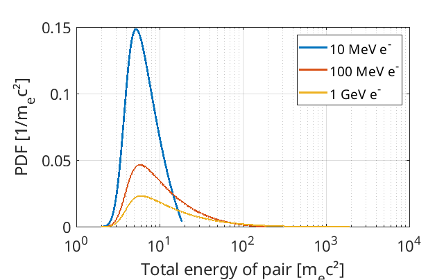
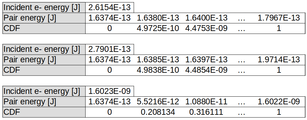
These PDFs may be integrated to obtain a CDF, which can be used for sampling. A pre-calculated CDF list is obtained for each incident energy considered, creating tables of the form given below:
Once the pair energy has been selected, the energy of the individual pair particles can be sampled in a similar way. Martinez (2019) uses a second differential cross-section in Eq. (31), equivalent to Bhabha (1935) Eq. (32). Since this expression will be normalised to form a PDF, then a CDF, the constant terms in Bhabha’s equation can be ignored, yielding:
\(\frac{d\sigma}{d\gamma_+} \propto \left( \gamma_+^2 + \gamma_-^2 + \frac{2}{3}\gamma_+\gamma_- \right) \ln\left( \frac{\gamma_+\gamma_-}{\gamma_p} \right)\)
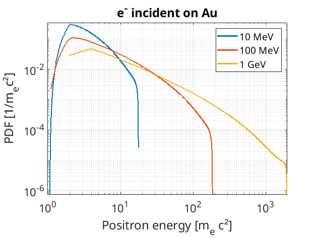
By muliplying the probabilities of each \(\gamma_+\) for a given \(\gamma_p\) by the probability of sampling \(\gamma_p\) itself, and summing over all possible \(\gamma_p\), we can obtain a \(\gamma_+\) PDF for a given incident \(e^-\) energy. A selection of these is given below:
In the code, EPOCH first calculates a \(\gamma_p\) from sampling, and then uses this to sample from a second set of tables based on \(d\sigma/d\gamma_+\). These tables are similar to those for pair-production, and a subset of values is given here:
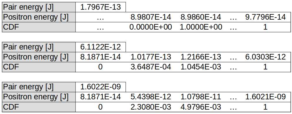
Note that \(d\sigma/d\gamma_+\) can sometimes go negative. If this happens, we assume the positron energy is invalid, and set the differential cross-section to zero. For some incident energies, \(d\sigma/d\gamma_+\) is always negative. When this happens, we have the CDF rise from 0 to 1 in the central values - giving electrons and positrons an equal energy split. An example of this is present in the above figure, for pair energy \(1.7967\times 10^{-13}\) J.
Angular distribution#
While it would be possible to use Eq. (27) in Bhabha (1935) to derive an angular distribution for emitted pairs, this has not yet been implemented in EPOCH. Instead, it is assumed that the momenta of the pair particles are parallel to the incident electron momentum direction.
Example: Nuclear trident#
In this example, \(5 \times 10 ^5\) \(e^-\) are initialised in the first 5 cells
on the x_min boundary, and are each set to an energy of 1 GeV. These \(e^-\)
propagate through 1 cm of solid-density Au, with the nuclear-trident process
switched on. Macro-particles created for the Electron and
Positron species are set to be immobile, such that their positions at the end
of the simulation describe where they were created.
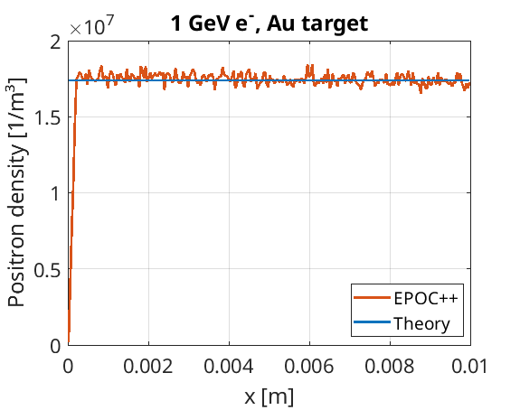
Using Martinez (2019) Eq. (26) for the nuclear-trident cross-section, 1 GeV \(e^-\) in gold have a cross-section of \(5.8 \times 10^{-28}\) m². For a gold target with density \(6.0 \times 10^{28}\) /m³, this corresponds to a pair-production rate of around \(1.06 \times 10^{10}\) /s.
Since the pair-energies tend to be much lower than the incident energy at 1 GeV, let us assume that the incident \(e^-\) energy change is negligible when pairs are produced. Hence, the pair-production rate may be approximated as constant for all incident electrons. This can be used to estimate the number density of immobile pairs as a function of depth, which has been modelled with EPOC++, and compared to theory:
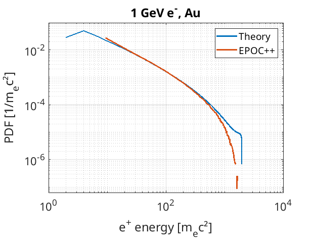
The energy spectrum of produced positrons was also calculated, and normalised to show a probability density function. This was then compared to the PDF expected by following the procedure in Martinez (2019), and it was found that the energy distribution had a good agreement with theory:
These plots were produced using the input deck below:
begin:control
  nx = 256
  x_min = 0
  x_max = 0.01
  t_end = 35e-12
  verbose = 2
  stdout_frequency = 10
end:control

begin:boundaries
  bc_x_min = open
  bc_x_max = open
end:boundaries

begin:physics_package
  process = nuclear_trident
  incident = Electron_in
  background = Gold
  electron_species = Electron
  positron_species = Positron
end:physics_package

begin:species
  name = Electron_in
  drift_x = 5.341e-19
  rho = 1.0e5 * nx / (x_max - x_min)
  rho = if (x lt 5*dx, density(Electron_in), 0)
  npart = 2048000
  identify:electron
end:species

begin:species
  name = Gold
  atomic_number = 79
  charge = 0
  mass = 359109
  rho = 6.0e28
  npart_per_cell = 2000
  immobile = T
end:species

begin:species
  name = Electron
  immobile = T
  identify:electron
end:species

begin:species
  name = Positron
  immobile = T
  identify:positron
end:species

begin:output
  name = rst
  nstep_snapshot = 10
  rolling_restart = F
  dump_first = T
end:output