Example 3: Field background#

The EPOCH physics packages can sometimes have rates which depend on the current field strength/direction interpolated over the macro-particle position. Hence, the interpolated fields need to be accessible when the packages run. To prevent recalculation, the cell-weighting factors are saved for each particle, as are the interpolated field values themselves.

The physics package test_process_EB_background was developed to demonstrate a process which uses background fields. The trigger rate is set to \(E_y^2\), interpolated over the macro-particle shape. When triggered, the z-component of the momentum is increased by 1e-23 kgm/s. This was chosen as a y-polarised laser in a 1D code cannot exert a force in the z-direction, so any momentum here must be created by this process. The background current density is also modified by this process, and +5.0e-13 A/m² is added to the grid at the particle position.

The test_process_EB_background runs in one of two ways, depending on whether the total_pz_transfer key is provided in the physics_package block.

Default behaviour: test_process_EB_background will apply a momentum shift to the particle each time it is triggered.
total_pz_transfer: if this key is used, a shared particle variable total_pz_transfer is created. All instances of test_process_EB_background stop when the total transferred pz is reached.

In these examples, a long electron plasma is initialised on the high-x side of the simulation window, and a laser is injected through the low-x side. The electrons may undergo the test_process_EB_background interaction, and the laser intensity is set such that the interaction rate is very high.

Two examples are provided for this system:

example_3_0: Electrons use test_process_EB_background
example_3_1: Two test_prcess_EB_background packages are used, but with a shared pz limit

Example 3.0#

The incident electrons start at rest, and the laser travels towards them from the low-x boundary. As the laser passes through the plasma, test_process_EB_background is rapidly triggered, and extra momentum is applied to the electron \(p_z\). This process will trigger most steps, and particles which spend longer in the laser field (those closer to the injection boundary) will gain the most \(p_z\).

The physics package block takes the form:

begin:physics_package
   process = test_process_EB_background
   incident = Electron_bunch
end:physics_package

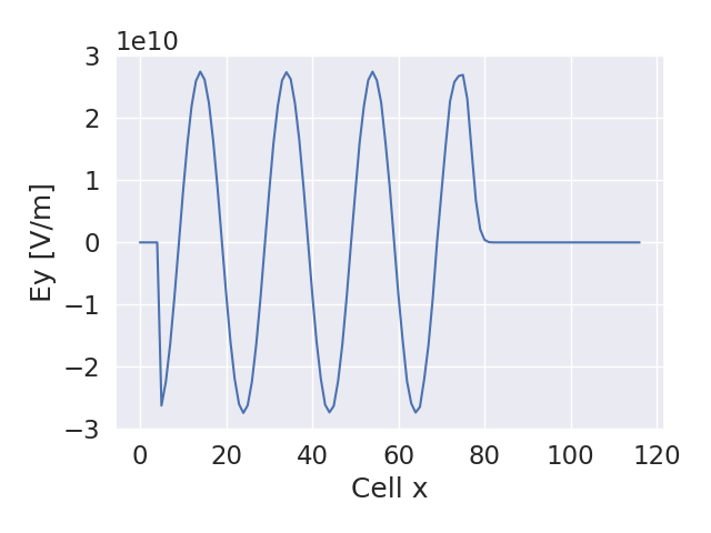
The laser moves through the simulation window from the low-x boundary, and at the simulation end, the laser fields are shown here:

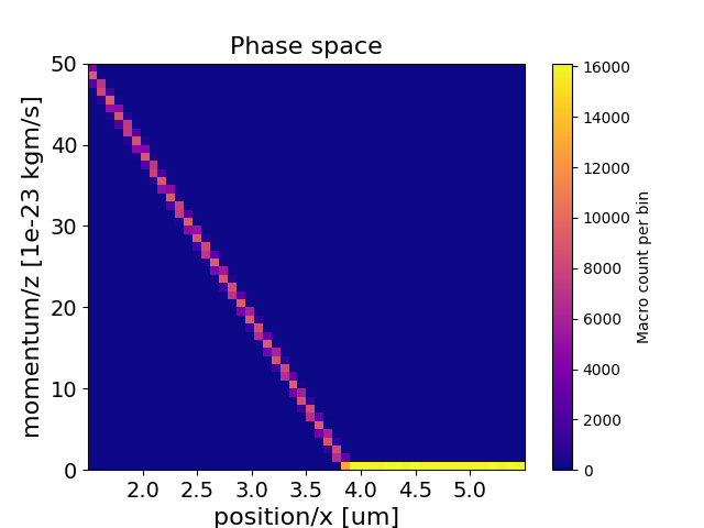
Ey electic field in each cell at the end of Example 3.0

We can see the effects of this package by plotting the \((x,p_z)\) phase space for the electrons. Electron \(p_z\) has a linear dependence on distance, which is directly related to how long each electron has spent in the laser field.

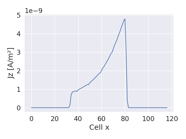
(x, pz) phase-space of electrons in the species Electron_bunch at the end of Example 3.0

When triggered, a positive \(J_z\) is added to the particle position, to compete with the negative \(J_z\) caused by the transferred momentum. This \(J_z\) will modify the field-solver, but will disappear when current is recalculated during the next Boris push. However, particles at lower \(x\) have gained more \(p_z\), so will have a greater negative \(J_z\) magnitude to counter the process-trigger positive \(J_z\). Hence, the positive \(J_z\) magnitude is lower in regions which have spent longer in the electric fields, as seen here:

Jz current density in each cell at the end of Example 3.0

Example 3.1#

This example applies two test_process_EB_background processes to the Electron_bunch species, but the momentum added to each particle is tracked with a shared particle variable. Both processes contribute to this variable, and both will switch off when the limit is reached.

The cut-off momentum chosen in this example is 5.0e-23 kgm/s:

begin:physics_package
   process = test_process_EB_background
   incident = Electron_bunch
   total_pz_transfer = 5.0e-23
end:physics_package

begin:physics_package
   process = test_process_EB_background
   incident = Electron_bunch
end:physics_package

When run, we see that the expected cut-off momentum is achieved:

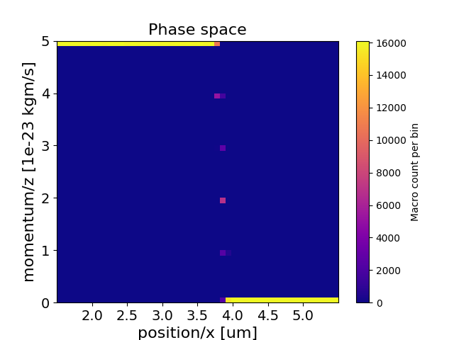
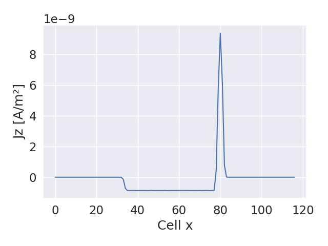
(x, pz) phase-space of electrons in the species Electron_bunch at the end of Example 3.1

Once this cut-off is reached, the process no longer runs, and positive \(J_z\) is no longer added to the particle position. Hence, when we look at the current density, we see a negative \(J_z\) calculated from the positive \(p_z\) of the electrons in this step. It’s only at the laser-front, where electrons have not yet reached the cut-off momentum, where the process is still triggering and a positive \(J_z\) is present.

Jz current density in each cell at the end of Example 3.1

Phase space plotter#

The Python script used to generate the above results is provided here:

import sys
sys.path.append('/home/stuart/Postdoc/EPOCpp/epc_readers')

from epc_parser import epc
import numpy as np
import matplotlib.pyplot as plt

core_count = 1
file_no = 80
spec_id = 1
path_to_data = "/home/stuart/Postdoc/Keith/EPOCpp/example_decks/Physics_package_examples/"
x_axis = "position/x"
y_axis = "momentum/z"

file_no_string = str(file_no).zfill(5)

# Obtain x positions of all particles
x_data = np.array([])
y_data = np.array([])
if (core_count > 1):
  for i in range(core_count):
    core_str = str(i).zfill(3)
    print(core_str)
    data = epc(path_to_data + "data" + file_no_string + "_" + core_str + ".epc")
    x_data = np.concatenate((x_data, data.get_array("/data/" + str(file_no) + "/particles/" + str(spec_id) + "/" + x_axis)))
    y_data = np.concatenate((y_data, data.get_array("/data/" + str(file_no) + "/particles/" + str(spec_id) + "/" + y_axis)))
else:
  data = epc(path_to_data + "data" + file_no_string + ".epc")
  x_data = data.get_array("/data/" + str(file_no) + "/particles/" + str(spec_id) + "/" + x_axis)
  y_data = data.get_array("/data/" + str(file_no) + "/particles/" + str(spec_id) + "/" + y_axis)

plt.hist2d(x_data * 1.0e6, y_data*1.0e23, bins=50, cmap='plasma')
plt.colorbar(label='Macro count per bin')
plt.xlabel(x_axis + " [um]", fontsize=16)
plt.ylabel(y_axis + " [1e-23 kgm/s]", fontsize=16)
plt.title("Phase space", fontsize=16)
plt.xticks(fontsize=14)
plt.yticks(fontsize=14)

# Show the plot
plt.show()

Current density plotter#

Finally, the Python script used to plot current densities is:

import sys
import os
import numpy as np
import seaborn as sns
import matplotlib.pyplot as plt
import matplotlib.ticker as ticker
from matplotlib.ticker import MaxNLocator

sys.path.append(os.path.abspath('/home/stuart/Postdoc/EPOCpp/epc_readers/'))
from epc_parser import epc

step = 80
core_count = 1
i_core = 2
path_to_data = "/home/stuart/Postdoc/Keith/EPOCpp/example_decks/Physics_package_examples/"
mesh = "J/z"
file_no_string = str(step).zfill(5)

if core_count == 1:
  data = epc(path_to_data + "data" + file_no_string + ".epc")
else:
  core_str = str(i_core).zfill(3)
  data = epc(path_to_data + "data" + file_no_string + "_" + core_str + ".epc")

field = data.get_array("/data/" + str(step) + "/meshes/" + mesh)
sns.set(font_scale=1.5)
plt.plot(field)
plt.xlabel("Cell x")
plt.ylabel("Jz [A/m²]")
plt.tight_layout()
plt.show()

Example 3: Field background

Contents

Example 3: Field background#

Example 3.0#

Example 3.1#

Phase space plotter#

Current density plotter#