Bethe-Heitler muon pair production

This process describes the decay of an incident photon into a muon-antimuon pair. The specific implementation in EPOCH follows that reported by Burkhardt, Kelner, and Kokoulin in a 2002 report, currently hosted by Cern with a report label: No. CERN-SL-2002-016-AP. This is the muon generation method used by Geant4, and the method in the Burkhardt report can also be found in the Geant4 Physics Reference Manual.

Cross sections

Burkhardt et al calculate the muon pair-production cross section by applying the quantum field theory crossing relations to the process of bremsstrahlung radiation from muons. They use this to obtain a parametrised cross section \(\sigma\), including field-screening effects from orbital electrons, in their Eq. (11):

\(\sigma = \frac{28 \alpha Z^2 r_c^2}{9} \log(1 + W_M C_f E_g)\)

Here, \(Z\) is the atomic number of the target, \(r_c\) is the classical muon radius (\(e^2/(4\pi\epsilon_0 m_\mu c^2)\)), for muon mass \(m_\mu\), and the other terms take the form:

\(W_M = \frac{10^9 e}{4 D_n \exp(0.5) m_\mu c^2}\)

\(C_f = 1 + 0.04 \ln\left(1 + \frac{10^9 e}{E_\gamma} \left(-18 + \frac{4347}{B}Z^{1/3}\right)\right)\)

\(E_g = \left( 1 - \frac{4 m_\mu c^2}{E_\gamma} \right)^t \left( \left( 4\times 10^{-9} B Z^{-1/3} \exp(0.5) \frac{m_\mu}{e m_e} m_\mu c^2 \right)^s + \left(\frac{E_\gamma}{10^9e}\right)^s\right)^{1/s}\)

where \(E_\gamma\) is the incident photon energy. In this documentation, the Burkhardt equations have been converted to SI units. The original Burkhardt report quotes these equations using units of GeV/c² for mass, and GeV for energies.

The above parametrisation has introduced new terms, which will be explained here. For hydrogen, we have:

\( B = 202.4\)

\(D_n = 1.49\)

and for all other elements, with mass number \(A\):

\(B = 183\)

\(D_n = 1.54 A^{0.27}\)

For all elements, the constants \(s\) and \(t\) take the form:

\(s = -0.88\)

\(t = 1.479 + 0.00799 D_n\)

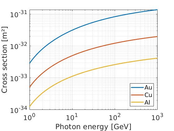
This parametrisation yields a cross-section which scales with incident photon energy, as shown here:

Pair particle energies

Burkhardt (2002) presents a differential cross section in their Eq. (2), which describes the distribution of \(x\), which represents the fraction of the photon energy going into one of the pair particles. This equation reads:

\(\frac{d\sigma}{dx} = 4 \alpha Z^2 r_c^2 \left(1 - \frac{4}{3} x(1-x)\right) \ln(W)\)

where \(W\) is given in Eq. (3) as:

\(W = Z^{1/3}\frac{B}{D_n} \frac{m_\mu}{m_e} \frac{2 E_\gamma x (1-x) + m_\mu c^2 (D_n \exp(0.5)- 2)}{2 E_\gamma x (1-x) + B Z^{-1/3}\exp(0.5) m_\mu^2 c^2 / m_e}\)

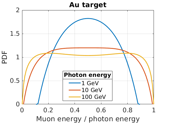
This differential cross-section can be calculated for a variety of \(x\) values for a fixed photon energy, and the resulting values can be normalised to form a PDF. This has been shown below for a variety of different incident photon energies:

Angular distribution

Burkhardt (2002) describes different forms of a multiply-differential cross-section used for sampling muon scatter variables. In practice, they propose steps to sample from this distribution in their Section 5. The method is too long to reproduce here, but an implementation may be found in the calc_bh_mu_kinematics function in src/physics_packages/bethe_heitler_mu.cpp.

Burkhardt provides example angular distributions from the sampling in their Figure 10, which may be used for verification of the procedure.

Example: Muon pair production

In this example, \(5 \times 10 ^5\) photons are initialised in the first 5 cells on the x_min boundary, and are each set to an energy of 100 GeV. These photons propagate through 500 m of solid-density Au, and the Bethe-Heitler \(\mu^-\mu^+\) process is switched on. Macro-particles created for the Muon and Anti species are set to be immobile, such that their positions at the end of the simulation describe where they were created.

Using Burkhardt Eq. (11), we calculate a pair-production cross section of \(8.26 \times 10^{-32} \text{ m}^2\) for 100 GeV photons in gold. This yields an expected rate of \(1.5\times 10^6 \text{ s}^{-1}\), which is constant for the simulated photons. Since each has a constant rate of decay, we expect an exponential distribution of survival depths. Each decay creates an immobile muon, and plotting the muon number density gives:

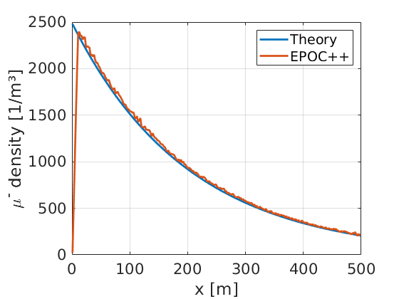
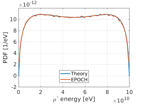
Here, it can be seen that the density of muons is as expected from theory, which suggests the code is calculating the correct decay rate. The energy distribution of the muons can also be calculated, which also agrees with the PDF expected from Burkhardt Eq. (2):

Finally, we can plot the scatter angle distribution of the muons. Here, \(\theta = 0\) corresponds to the positive \(x\) direction, and the \(\theta\) angle considers the momentum direction of the created particle. The result looks similar to the 100 GeV case given in Figure 10 of Burkhardt.

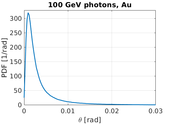
For a muon with typical energy 50 GeV, the Lorentz factor would be around \(\gamma \approx 470\), so \(1/\gamma \approx 0.002\). Here it can be seen that the scatter angle \(\theta \approx 1/\gamma\), as expected.

begin:control
  nx = 256
  x_min = 0
  x_max = 500
  t_end = 1.7e-6
  verbose = 2
  stdout_frequency = 10
end:control

begin:boundaries
  bc_x_min = open
  bc_x_max = open
end:boundaries

begin:physics_package
  process = bethe_heitler_mu
  incident = Photon_bunch
  background = Gold
  muon_species = Muon
  antimuon_species = Anti
end:physics_package

begin:species
  name = Photon_bunch
  drift_x = 5.341e-17
  rho = 1.0e5 * nx / (x_max - x_min)
  rho = if (x lt 5*dx, density(Photon_bunch), 0)
  npart = 2048000
  identify:photon
end:species

begin:species
  name = Gold
  atomic_number = 79
  charge = 0
  mass = 359109
  rho = 6.0e28
  npart_per_cell = 2000
  immobile = T
end:species

begin:species
  name = Muon
  immobile = T
  identify:muon
end:species

begin:species
  name = Anti
  immobile = T
  identify:antimuon
end:species

begin:output
  name = rst
  nstep_snapshot = 10
  rolling_restart = F
  dump_first = T
end:output