Sampling methods

This section provides the theory for the sampling methods used in EPOCH. This is the framework used for almost all the EPOCH processes. The exception is elastic collisions, which triggers too quickly to model each collision individually. The workaround here is to estimate the number of trigger events over a given time-step, and to sample a cumulative collision angle based on that number. All other processes are described by the optical depth method, which will be discussed in this section.

Event trigger probability

All standard physics packages in EPOCH are described by two things: a rate for the process to trigger \(\lambda\), and some kinematics behaviour for when the process does trigger. The rate is defined such that the probability of trigger over some small time, \(dt\), is given by:

\(P(dt) = \lambda dt\)

Hence, the probability that the event doesn’t trigger over \(dt\) is simply:

\(\bar{P}(dt) = 1 - \lambda dt\)

If we define a longer period of time as \(\Delta t = n dt\), then the probability of no-trigger over \(\Delta t\) is the same as no-trigger over \(dt\), \(n\) times back-to-back:

\(\bar{P}(\Delta t) = (1 - \lambda \frac{\Delta t}{n})^n\)

where we have written \(dt\) as \(\frac{\Delta t}{n}\). In the limit of infinitesimal \(dt\), we have \(n\rightarrow \infty\), and using the definition

\(\lim_{n\rightarrow \infty}\left(1 + \frac{x}{n}\right)^n = e^x\)

we have

\(\bar{P}(\Delta t) = e^{-\lambda \Delta t}\)

Hence, the probability that the process does trigger over \(\Delta t\) is:

\(P(\Delta t) = 1 - e^{-\lambda \Delta t}\)

This is the probability we attempt to sample in EPOCH, once the process rate \(\lambda\) is calculated. The parameter \(\Delta t\) will be the simulation time-step by default, but it could be multiple time-steps if the process is only sampled once every few time-steps. If the process rate is artificially increased, this factor is applied to \(\Delta t\). Each physics process will store its own \(\Delta t\) variable.

Optical depth method

Let us introduce the concept of an optical depth, \(\tau\), where

\(\tau(t) = \int_0^t \lambda(t') dt'\)

and the probability of a trigger by optical depth \(\tau\) is

\(P(\tau) = 1 - e^{-\tau}\)

When the optical depth travelled is 0, \(P(0) = 0\), and there is no chance of a trigger. As \(\tau\rightarrow\infty\), the probability of a trigger \(P(\tau)\rightarrow 1\). Let us re-arrange this expression to obtain:

\(\tau = -\ln\left(1 - P(\tau)\right)\)

The probability \(P(\tau)\) actually describes a cumulative density function, and from this we may sample a trigger optical depth \(\tau_d\). If we replace \(P(\tau)\) with a uniformly-distributed random number between 0 and 1, \(x_r\), we get:

\(\tau_d = -\ln x_r\)

Here, we have used the fact that \((1-x_r)\) is also equivalent to a uniformly distributed random number between 0 and 1, so we sample from this.

A trigger optical depth is sampled for each particle at the start of the simulation (for each active process), and is stored in an optical-depth particle variable, \(\tau\). Initially, \(\tau = \tau_d\) for each particle, and this variable describes the remaining optical depth to travel before the process triggers. Each time the process runs, we perform:

\(\tau(t) = \tau(t_\text{previous}) - \lambda(t) \Delta t\)

and when \(\tau(t) < 0\), the process triggers. Depending on the physics package, this may destroy the incident particle (like a photon in pair-production). If the incident particle survives, it may perform the process again (an electron can radiate more than one bremsstrahlung photon).

If a process can be triggered more than once, then a new trigger optical depth \(\tau_d\) is sampled whenever a process triggers. At this point, \(\tau(t)\) is a negative number. Physically, this negative number represents optical depth travelled towards the next trigger point. If we add our new \(\tau_d\) to the current negative \(\tau\), then the “overshoot” from the current step is applied, and we may proceed as normal. However, there are two complications to consider:

• The negative \(\tau\) was calculated using the rate before the process triggered. The rates of physics packages typically scale with the incident particle energy, which can change when the process triggers. Hence, this overshoot will not be fully correct.

• Suppose the overshoot was large, and the newly sampled \(\tau_d\) is small. We may find that \(\tau(t) + \tau_d\) is still negative, which would suggest the process must trigger on the next step too. However, if the rate, \(\lambda\), of the next step is 0, then a trigger would be non-physical. Hence, for a process to trigger, we must have \(\tau<0\) and \(\lambda > 0\).

When reading the “unfinished work” section, I describe a super-cycling extension which would remove these two complications. This may come at the expense of computational performance though.

Physically increased rates

In a standard physics package, the weight of created secondary macro-particles matches the incident macro-particle weight. However, sometimes the user may wish to model rare processes, where the number of real secondary particles is considerably lower than the number of real incident particles. In these cases, waiting for the creation of a secondary macro-particle which matches the incident weight could take a long time, and lead to poor statistics.

Instead, we will provide a user with the ability to separate the secondary emission behaviour from the incident trigger behaviour. The process rate may be scaled up or down by the user, which affects the code in different ways.

If the rate is increased by some factor, \(n\), this is applied within the code to \(\Delta t\). The process will trigger more often, and a secondary macro-particle will always be created, but with weight reduced by a factor of \(n\) to conserve the number of real secondaries. The incident macro-particle will only trigger with a probability \(1/n\), to ensure the distribution of incident trigger-points is the same. When an event is triggered, the code separately tracks whether an incident particle was triggered, a secondary particle was triggered, or both.

As an example, we constructed a toy system to mimic pair production. We started with \(10^6\) real electrons, and they had a 2% chance to create a pair each step. After running multiple steps, we had a distribution of pair creation as a function of step number, as seen below.

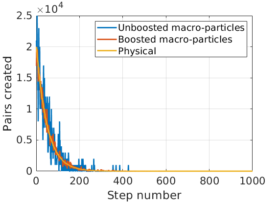
This was repeated using \(10^3\) macro-electrons, each with a 2% decay chance per step, creating pairs of the same weight. This matched the physical curve, but was noisier. Finally, \(10^3\) macro-electrons were tracked with an \(n=10\) boost - following the above procedure produced the same distribution as the physical case, but with less noise and improved statistics.

Weighted collisional processes

In collisional processes where incident and background particles are both affected, we require a scheme to ensure the correct number of real incident and background particles are triggered.

Suppose a cell contains macro-electrons of weight \(W_1\), and macro-ions of weight \(W_2\). Each real electron described by the macro-electron may have a reaction probability of \(P(\Delta t)\), which means that on average, the macro-electron should trigger \(N_2 = W_1 P(\Delta t)\) reactions. Let us consider the scheme shown here:

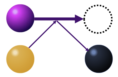
when the collision-process triggers, our incident electron (purple) is destroyed, and the ion (yellow) changes into a different particle (black). This is equivalent to an electron recombination process.

If we have an incident macro-electron of weight \(W_e = 100\) and \(P(\Delta t) = 0.1\), then we expect 10 real electrons to be destroyed, and \(N_2=10\) real ions to change species. Let there be many macro-ions in the cell, each with \(W_i=4\). The method for triggering each macro-particle is performed as shown in this diagram:

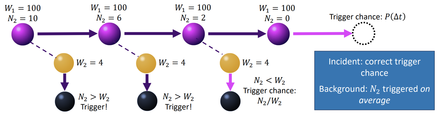
Here, the macro-electron is paired with the first macro-ion. We require 10 real ions to change species, and the first macro-ion has a weight of 4. We will therefore trigger this macro-ion, but we still need another 6 real ions to change species, so we consider the next macro-ion. Again, the weight is 4, and we need 6 triggers, so we trigger the second macro-ion. For the third macro-ion, the weight is 4, but we only need 2 more triggers. To get the correct number of triggered particles on average, we only trigger this final macro-ion with a probability of \(N_2^\text{remaining} / W_2 = 0.5\). Once the macro-ions have been sampled, we perform the macro-electron sample. Here, we only trigger the macro-electron behaviour with the reaction probability \(P(\Delta t) = 0.1\), which destroys the correct number of macro-electrons when averaged over many macro-particles.

Cumulative density functions

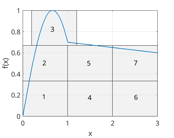
Quite often, physics packages involves sampling numbers from distributions - mainly for calculating the energies of newly created secondary particles. To do this, we’ll sample from cumulative density functions. To demonstrate how this works, consider sampling from this simple function.

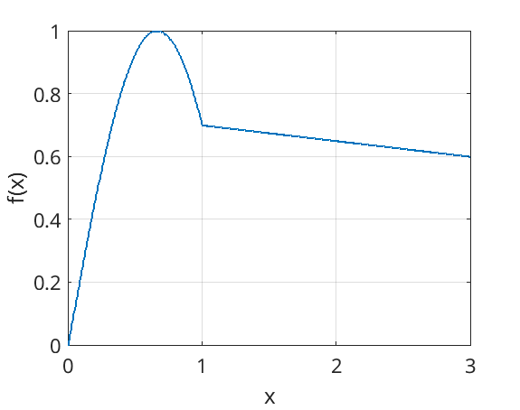
If we break this function down into equally sized boxes, and label these 1-7, then we can produce a decent approximation of this function by randomly picking a number between 1 and 7, and returning the \(x\) value of the corresponding box.

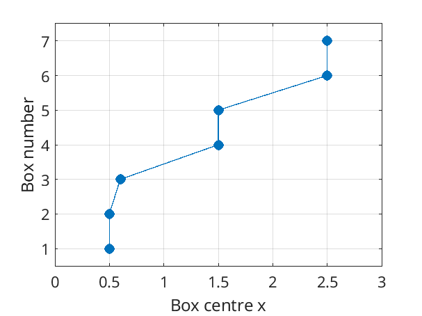
This procedure may be better illustrated if we considered plotting \(x\) against box number. By repeatedly picking random points on the vertical axis, and finding the corresponding point on the \(x\) axis, we will eventually reproduce the original distribution.

The cumulative density function (CDF) approach takes this idea, but uses many, infinitesimally small boxes. A normalisation is provided such that the vertical axis scales between 0 and 1. The CDF function \(C(x)\) may be calculated for a function \(f(x)\) by using:

\(C(x) = \frac{\int_{x_0}^{x} f(x')dx'}{\int_{x_0}^{x_1} f(x')dx'}\)

where \(f(x)\) is defined between \(x=x_0\) and \(x=x_1\). In our example, this produces the plot seen here:

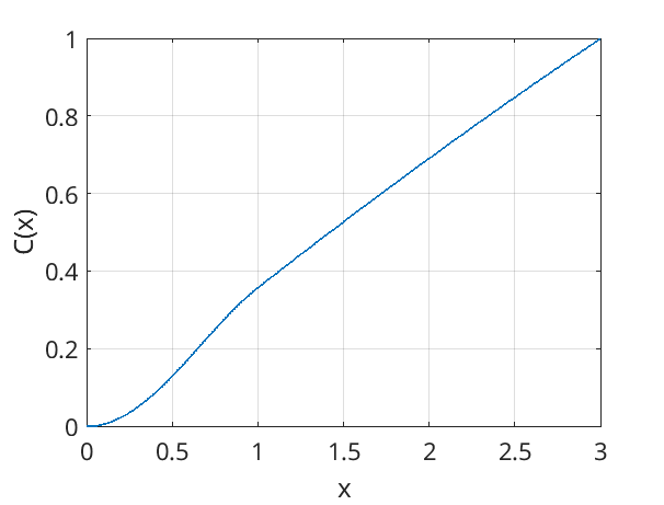
It can be seen that this plot represents a higher-resolution version of the previous boxy approximation. If we sampled points on the vertical using a uniformly-distributed random number between 0 and 1, and found the corresponding \(x\) value, we would accurately reproduce the distribution function \(f(x)\).