Collisional ionisation

The collisional ionisation method in EPOCH follows the methods described in Morris (2022) Physics of Plasmas, 29(12). This is a part of the collisional ionisation and recombination package, which pairs incident and background macro-particles together, and can modify the properties of both particles.

The ionisation/recombination package calculates the rates of both ionisation and recombination, subtracts one from the other to determine the net change, and applies the dominant process. If collisional ionisation dominates, the background ion is moved to a species with a higher charge state, a new electron macro-particle is created, and the incident electron has its momentum reduced to conserve energy and momentum. No angular emission model has been used, so the ejected electron travels in the direciton of the incident electron.

Ionisation tables

There are 6 categories of table present in the EPOCH source-code, which are used in ionisation packages to characterise different ion species with different charge-states and atomic numbers. These can be found in include/physics_packages/tables.

The first 3 tables contain data for all elements, and all their charge-states. Each row describes an ion with a different atomic number \(Z\), and the columns are related to the ion-charge-state (including neutral). These tables describe the ionisation energy of the ion, and the \(n\), \(l\) quantum numbers of the outermost bound electron. Ionisation energies are taken from the “NIST Atomic Spectra Database (Ionization Energies Data)”, Kramida et al (2024).

This database also provides the ground-state electron configuration of each ion-state. By inspecting the change in ground-state configurations between subsequent ions, we can deduce which electron has been liberated - this is taken to be the “outer-electron”. Sometimes there is ambiguity, as multiple electrons change between ground-state configurations. For example, the ground-state of neutral V is written \([\text{Ar}]3d^3 4s^2\), while \(\text{V}^+\) has \([\text{Ar}]3d^4\). Here, both \(4s^2\) electrons have vanished, one ionised, the other removed to \(3d\). In all cases where more than one bound electron is affected, these multiple electrons always come from the same shell - we can still identify a single shell for outer \(n\) and \(l\) numbers.

Ionisation energies are given in units of eV, and a sample of values from the EPOCH file ionisation_energies.table is given below:

We use the same table format for the outer quantum numbers. The outer \(n\) quantum numbers are found in ion_n.table, and the first few lines read:

Similarly, for the \(l\) quantum number, the first few lines of ion_l.table read:

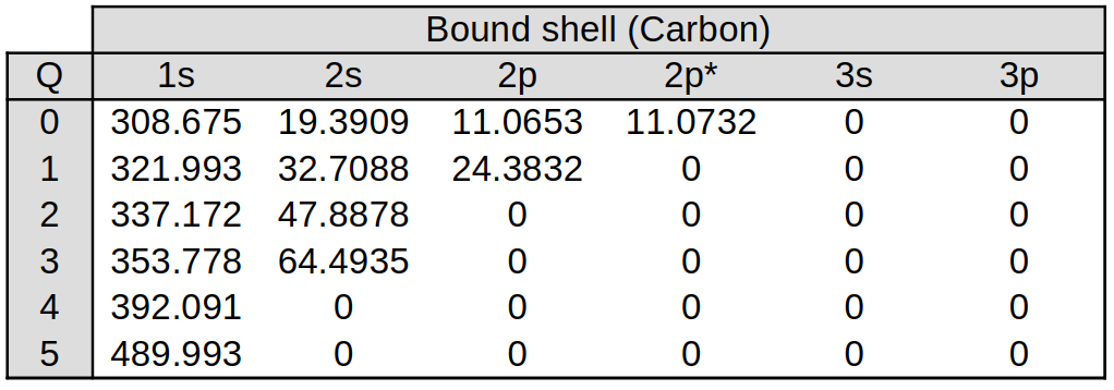
The next three tables follow a different format, where each element is given its own file. Here, each line represents a different ion-charge-state, and columns represent different bound electron shells. These tables give the binding energies of electrons bound in each shell, along with their mean bound kinetic energy, and sometimes the number of bound electrons in each shell.

The binding energies are found in the binding_energy directory, and the files take the format be_Z, where \(Z\) is replaced with the element atomic number. The binding energies for neutral atoms were transcribed from Table 2 of Desclaux (1973) At. Data Nucl. Data Tables, 12(4), 311-406. For charged ions, the Desclaux binding energies were modified following Eq. (4) of Carlson (1970) At. Data Nucl. Data Tables, 2, 63-99:

\(B_{nl}(Q) = I(Q) - B_{nl\text{,outer-Q}}(Q=0) + B_{nl}(Q=0)\)

where \(B_{nl}(Q)\) is the binding energy of shell \(nl\) in an ion with charge-state \(Q\), \(I(Q)\) is the ionisation energy of the same ion, and the subscript \(nl\text{,outer-Q}\) refers to the outermost shell of the ion with charge-state \(Q\). Terms with \(Q=0\) refer to the neutral atom, and these values are taken from Desclaux (1973).

There is limited tabulated data on the mean-kinetic-energy of bound-electrons, \(U_{nl}\), so in most cases, EPOCH uses the approximation \(B_{nl} = U_{nl}\). An analysis of this approximation is present in Morris (2022). This approximation means that most of the \(B_{nl}\) and \(U_{nl}\) files are identical, but they are kept separate in case users wish to calculate their own \(U_{nl}\) values. These files can be found in the bound_ke directory, with file-names in the u_Z format. At the time of writing, pre-calculated \(U_{nl}\) values have only been given for Au, which were provided by the NOVA school of science and technology in Portugal, using the mdfgme code.

A sample of values from the be_6 (and the identical u_6) tables are given below, which provide energies in units of eV:

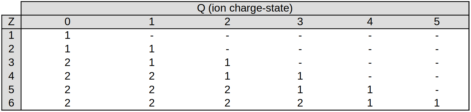
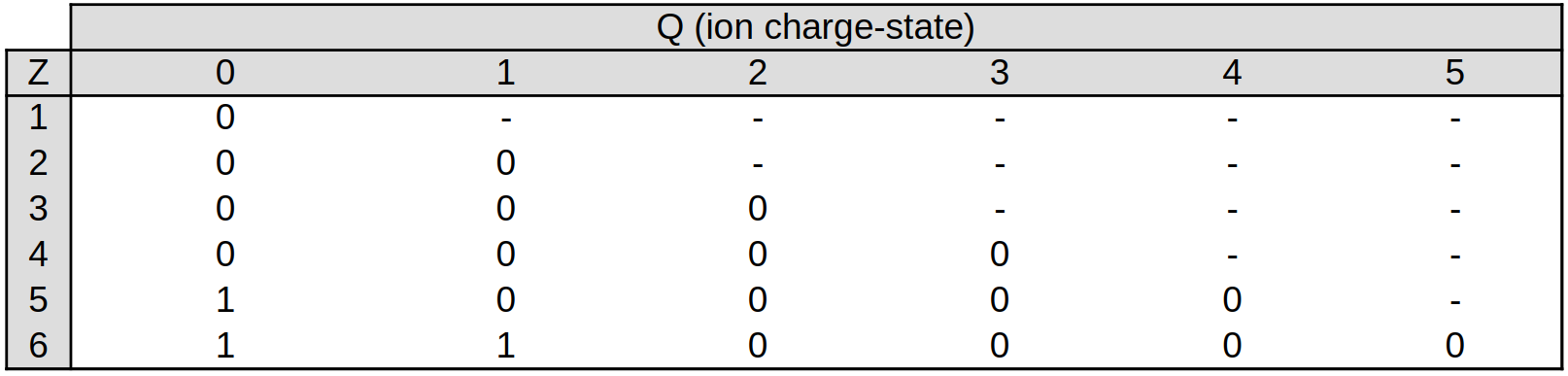
Using the atomic number and the charge-state, EPOCH can determine how many bound electrons are present. By default, the code will assume these bound electrons fill shells in the order provided by Eq. (4) of Morris (2022):

\(1s, 2s, 2p, 2p^∗ , 3s, 3p, 3p^∗ , 4s, 3d, 3d^∗ , 4p, 4p^∗, 5s, 4d, 4d^∗,\)

\(5p, 5p^∗ , 6s, 4f, 4f^∗ , 5d, 5d^∗ , 6p, 6p^∗ , 7s, 5f, 5f^∗ , 6d, 6d^∗\)

only moving onto the next shell when the previous is filled. Since the shells with \(l>0\) are split into two subshells, we assume each can only hold \((l+1)\) electrons. Shells with \(l=0\) can hold 2 electrons.

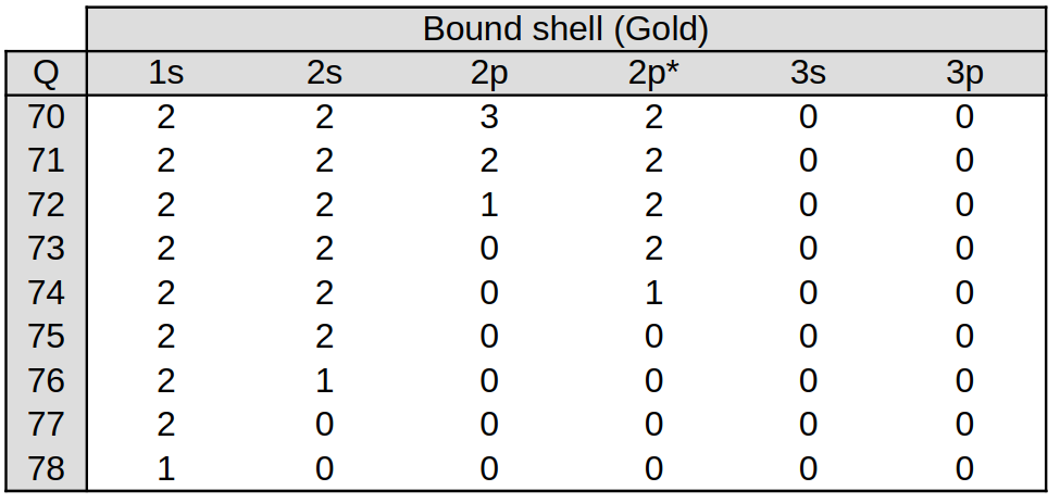
When the \(U_{nl}\) values were calculated for Au, it was found that this basic ground-state model was inconsistent with the results of mdfgme, which placed the bound electrons in different shells. Hence, EPOCH allows this basic shell structure to be overriden if the number of bound electrons in each shell is known. EPOCH will search for the existence of a table in occupancy_numbers, with the file-name occ_no_Z for atomic number \(Z\). If found, these occupancy numbers are used, otherwise the code will default to Morris (2022) Eq. (4). At present, such a table only exists for Au. The final few lines of occ_no_79 are provided here:

Cross sections

EPOCH uses one of two collisional ionisation cross-section models, depending on the atomic number of the target. As discussed in Section IIIB of Morris (2022), the MBELL method includes an empirical fit to experimental data, and so it will provide closer cross-sections to experimental observations in targets where the fit has been performed (atomic number \(Z < 19\)). For targets with higher atomic numbers, the MBELL method cannot be used, and the RBEB method is chosen instead. Details on these methods will be provided in later sections.

The cross-sections are pre-calculated during simulation setup for whichever targets are present. One hundred incident electron kinetic energies are logarithmically sampled from the minimum target binding energy, to 1 GeV. The total collisional ionisation cross-section corresponding to each incident energy, including contributions from all bound electrons present in the target, are stored in a second table.

An example of the table format is given below, calculated for a neutral nitrogen target.

Each bound electron contributes to the cross-section for collisional ionisation, and so ions with many loosely-bound electrons will tend to have higher cross-sections than those with only a few strongly-bound electrons. The cross sections for a few example species have been calculated here, using MBELL for \(Z<19\), and RBEB otherwise:

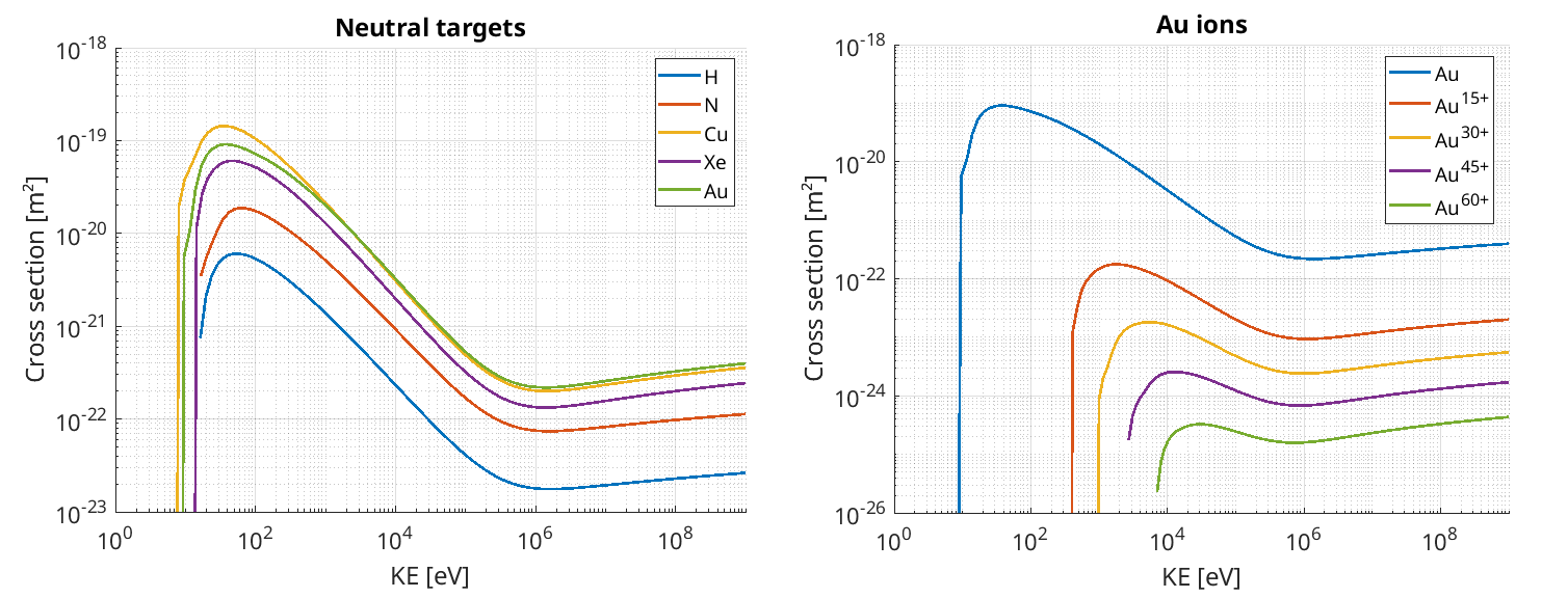
The methods used to calculate these cross-sections will be given in the following sections.

MBELL method

The modified-Bell (MBELL) model is documented by Haque (2006) “Electron impact ionization of M-shell atoms” Physica Scripta 74.3, and a summary of the method is present here. Details on the specific implementation in EPOCH are given by Morris (2022). MBELL uses fits to experimental data to calculate the cross section contributions of bound electrons for \(n\leq 3\), \(l \leq 2\). While the model can calculate bound-shell contributions from the \(3d\) shell, bound electrons typically occupy the \(4s\) shell before this, so only targets with bound electrons up to the \(3p\) shell can be fully described by MBELL. Hence, this model is used for \(Z < 19\).

The MBELL cross-section is given in Haque (2006) Eq. 1. Here, the cross-section contribution for a single bound electron reads:

\(\sigma_{nl} = F_\text{ion} G_r \sigma_\text{BELI}\)

Note that the MBELL paper considers all bound electrons in a shell at once. This is different to the EPOCH implementation, but equivalent. The total collisional ionisation cross-section is the sum of all the bound-electron contributions.

The term \(F_\text{ion}\) corrects for the target charge-state, and takes the form given in Haque (2006) Eq. (4):

\(F_\text{ion} = 1 + 3 \left( \frac{Z - N_u}{UZ} \right)^{\lambda(l)}\)

where \(\lambda\) changes with shell quantum number \(l\): \(\lambda(l=0) = 1.270\), \(\lambda(l=1) = 0.542\). Also, \(U = \epsilon_k / B_{nl}\), which describes the ratio of incident kinetic energy \(\epsilon_k\) to the binding energy of the current shell \(B_{nl}\). \(N_u\) is the number of bound electrons up to and including the current shell - for a bound electron in the \(2s\) shell, this would be 4 if both the \(1s\) and \(2s\) shells are full. Shells are considered the same if they share an \(nl\), so \(2p\) and \(2p^*\) are treated as a single shell in the \(N_u\) calculation.

\(G_r\) is given by Haque (2006) Eq. (3), which gives:

\(G_r = \frac{1 + 2J}{U + 2J} \left(\frac{U + J}{1 + J} \right)^2 \left(\frac{(1+U)(U+2J)(1+J)^2}{J^2(1+2J) + U(U+2J)(1+J)^2}\right)^{1.5}\)

where \(J = m_e c^2 / B_{nl}\).

Finally, \(\sigma_\text{BELI}\) is given by Haque (2006) Eq. (2), and reads:

\(\sigma_\text{BELI} = \frac{1}{B_{nl}\epsilon_k} \left( a(n,l) \ln\left(\frac{\epsilon_k}{B_{nl}}\right) + \sum_{K=1}^7 b_K(n,l)\left(1 - \frac{B_{nl}}{\epsilon_k}\right)^K\right)\)

where the fit parameters \(a(n,l)\) and \(b(n,l)\) are given in Haque (2006) Table 1, and are transcribed here in units of \(10^{-13} \text{eV}^2\text{cm}^2\):

\(nl\)	\(a\)	\(b_1\)	\(b_2\)	\(b_3\)	\(b_4\)	\(b_5\)	\(b_6\)	\(b_7\)
\(1s\)	0.525	-5.10	0.200	0.050	-0.025	-0.100	0.0	0.0
\(2s\)	0.530	-4.10	0.150	0.150	-0.200	-0.150	0.0	0.0
\(2p\)	0.600	-4.00	-0.710	0.655	0.425	-0.750	0.0	0.0
\(3s\)	0.130	0.250	-1.50	2.400	3.220	-3.667	0.0	0.0
\(3p\)	0.388	-0.200	-0.2356	0.5355	3.150	-8.500	5.05	0.37

RBEB method

The relativistic binary-encounter Bethe (RBEB) model combines various theoretical cross-sections, and is discussed in Kim (2000) Phys. Rev. A 62, 052710. The form used for EPOCH combines cross-sections from Eq. (22) and (37) in Kim (2000), which is written compactly in Eq. (8)-(12) in Morris (2022):

\(\sigma_{nl} = a_{nl} b_{nl} \left( c_{nl} \left( 1 - \frac{1}{t^2}\right) + d_{nl} \right)\)

with terms:

\(a_{nl} = \frac{1}{2}\left( 1 + \frac{\beta_t^2 + \beta_u^2 + \beta_b^2}{\beta_t^2} \right)\)

\(b_{nl} = \frac{2\pi a_B^2 \alpha^4}{(\beta_t^2 + \beta_u^2 + \beta_b^2)b'}\)

\(c_{nl} = \frac{1}{2}\left( \ln\left( \frac{\beta_t^2}{1 - \beta_t^2}\right) -\beta_t^2 - \ln(2b') \right)\)

\(d_{nl} = 1 - \frac{1}{t} - \frac{\ln(t)}{t + 1}\frac{1 + 2t'}{(1 + 0.5 t')^2} + \frac{b'^2(t-1)}{2(1 + 0.5 t')^2}\)

Here, \(\alpha\) is the fine structure constant, and \(a_B\) is the Bohr radius. We also have:

\(t = \frac{\epsilon_k}{B_{nl}}\)

\(t' = \frac{\epsilon_k}{m_e c^2}\)

\(b' = \frac{B_{nl}}{m_e c^2}\)

\(\beta_t^2 = 1 - \frac{1}{(1+t')^2}\)

\(\beta_b^2 = 1 - \frac{1}{(1 + b')^2}\)

\(\beta_u^2 = 1 - \frac{1}{(1 + U_{nl}/(m_e c^2))^2}\)

for an incident electron with kinetic energy \(\epsilon_k\).

Ejected electron energies

When an ion macro-particle undergoes collisional ionisation, it is moved to a species with a higher charge-state, and a new electron macro-electron is created to represent the ejected electron. Whether MBELL or RBEB is used to calculate the collisional ionisation cross-section, the method used to sample the ejected electron energy is the same, and is discussed in Section IIIC of Morris (2022). While Kim (2000) does not provide a differential cross-section for the RBEB method, an equation is derived in Eq. (14) of Morris (2022):

\(\frac{d\sigma_{nl}}{d\epsilon_\delta} = a_{nl} b_{nl} \left(-\xi_1(w) \frac{1}{t + 1}\frac{1 + 2t'}{(1 + 0.5 t')^2} + 2 c_{nl} \xi_3 (w) + \xi_2(w) + \frac{b'^2}{(1 + 0.5t')^2} \right)\)

where

\(\xi_i(w) = \frac{1}{(w + 1)^i} + \frac{1}{(t - w)^i}\)

\(w = \frac{\epsilon_\delta}{B_{nl}}\)

and \(a_{nl}\), \(b_{nl}\) and \(c_{nl}\) have the same form as used for the RBEB calculation. This documentation corrects a typo in the Morris (2022) manuscript, where \(b'^2\) is falsely written as \(bt^2\). Here, \(\epsilon_\delta\) is the kinetic energy of the ejected electron. As electrons are indistinguishable, the “ejected” electron is always taken to be the electron with the lower energy after the ionisation, with the “incident” electron having higher energy.

This function is sampled by calculating a cumulative distribution function (CDF) following Eq. (17) of Morris (2022):

\(\text{CDF} = a_{nl} b_{nl} \left[ \left( \frac{1}{(t-w)^2} - \frac{1}{(w+1)^2} - \frac{1}{t^2} + 1 \right)c_{nl} + \left(\frac{1}{t - w} - \frac{1}{w + 1} -\frac{1}{t} + 1\right)\right.\)

\( + \left.\frac{b'^2 w}{(1 + 0.5 t')^2} - \ln\left(\frac{t(w+1)}{t - w}\right)\left(\frac{1}{t+1}\right)\left(\frac{1 + 2t'}{(1 + 0.5t')^2}\right)\right]\)

These CDF values are calculated at the start of the simulation, evaluated at 20 logarithmically spaced \(\epsilon_\delta\) points between 0.01 eV and the maximum ejected kinetic energy, \(0.5 (\epsilon_k - B_{nl, \text{min}})\), where \(B_{nl, \text{min}}\) is the lowest binding energy of all bound electrons in the ion. This maximum energy corresponds to an equal split between the incident and ejected electron energy, after the binding energy has been subtracted. This comes from the condition that the “ejected” electron label is always applied to the lower-energy electron. A sample of ejected CDF tables is given here, for different initial incident kinetic energies \(\epsilon_k\) in neutral N targets

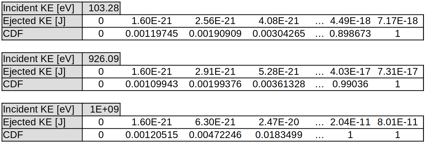
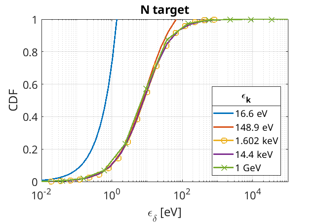
Also, since the first incident electron energy sampled refers to the case where the ejected electron is created with 0 energy, all \(\epsilon_\delta\) for this \(\epsilon_k\) are set to zero, with the CDF set to 1 for all but the first entry, which is 0. This forces the code to return a 0 ejected energy regardless of the sampled CDF. A sample of CDF curves are provided for different energies here, in a similar way to Figure 5 in Morris (2022):

Incident electron recoil

When an incident macro-electron is triggered in a collisional ionisation event, its kinetic energy is reduced by \(\epsilon_\delta + \langle B \rangle\), where \(\langle B \rangle\) is the cross-section-weighted mean binding energy of the target. This treatment is needed as EPOCH uses the total collisional ionisation cross-section, so we don’t know which shell the ejected electron emerges from. In the current EPOCH implementation, the momentum direction of the incident electron remains fixed.

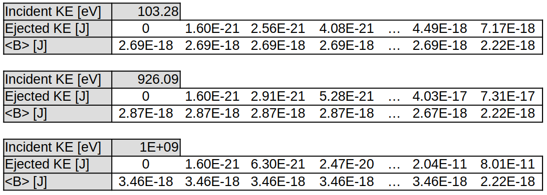
The mean binding energy is calculated using Eq. (5) of Morris (2022):

\(\langle B \rangle = \frac{\sum_{nl} N_{nl} \sigma_{nl} B_{nl}}{\sum_{nl} N_{nl} \sigma_{nl}}\)

where \(\sigma_{nl}\) is the cross-section contribution of a bound electron in shell \(nl\), \(N_{nl}\) is the number of bound electrons in this shell, and \(B_{nl}\) is the shell binding energy. This \(\langle B \rangle\) value is calculated for each pair of \(\epsilon_k\) and \(\epsilon_\delta\) values, and the sum is performed over every shell which satisfies \(B_{nl} > \epsilon_k - \epsilon_\delta\). This gives the binding energy averaged over every shell which the incident electron is capable of ionising into an outgoing energy \(\epsilon_\delta\), weighted by the probability of ejection from that shell. In EPOCH, the \(\sigma_{nl}\) values for each bound electron are saved during the computation of the total cross section for both the MBELL and RBEB models, and these are re-used in this calculation.

In practice, for a neutral N target, these tables take the form:

Example: Collisional ionisation

This example simulated a 1D periodic window, with uniformly distributed electrons and neutral Cu atoms. The electron species was set to a density of \(1\times 10^{27} \text{ m}^{-3}\), while the Cu species had density \(6\times 10^{28} \text{ m}^{-3}\). The electron kinetic energy was set to 10 keV (propagating in the \(x\) direction), and the macro-electron charge was set to zero. This non-physical charge was used to ensure incident electrons were unaffected by EM fields, such that any change in momentum was only due to the collisional ionisation process. The Cu species was set to be immobile, as were the additional \(\text{Cu}^+\) and ejected-electron species.

For 10 keV electrons in neutral Cu, the collisional ionisation cross section is around \(\sigma = 3\times 10^{-21} \text{ m}^2\). The Cu number density was initially \(n_i(t=0) = 6\times 10^{28} \text{ m}^{-3}\), and 10 keV electrons have a speed of \(v = 5.8 \times 10^{7} \text{ ms}^{-1}\). These numbers combine to give an initial ionisation rate of around \(10^{16} \text{ s}^{-1}\). A theoretical prediction for the change of \(n_i\) over some time interval \(\Delta t\) can be approximated as:

\(\Delta n_i = - n_e \sigma v n_i(t) \Delta t\)

which can be compared to the EPOCH results. The change in species number density over time is given here:

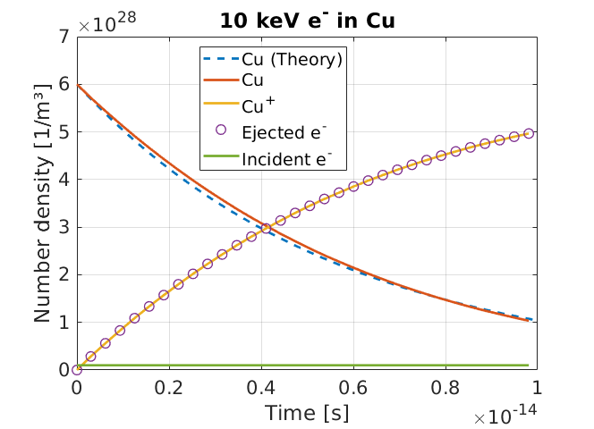
where the theoretical curve assumes \(\sigma\) and \(v\) are fixed over the simulation run-time. As incident electrons lose energy to ionising bound electrons, the speed and cross-sections will change over time, so an exact fit to this simple theory is not expected.

Since ejected electrons are held as immobile, the final energy distribution of the ejected electron species will match the energy distribution upon creation, which we can compare to the RBEB differential cross section quoted in a previous section. This comparison is made below, where it can be seen the ejected electron energies are sampled as expected:

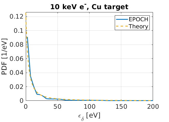
From the theory PDF curve, the average ejected electron kinetic energy should be around 27 eV in this system. The mean binding energy is around 15 eV for most ejected electron energies, in collisions between 10 keV electrons and neutral copper. Hence, each collisional ionisation event should remove around 42 eV from the incident electron. From the number density figure, it can be seen that by the end of the simulation, an incident electron population with density \(10^{27} \text{ m}^{-3}\) has created an ionised \(\text{Cu}^+\) population of density near \(5 \times 10^{28} \text{ m}^{-3}\). This implies each real electron triggers collisional ionisation around 50 times on average. With a typical energy loss of 42 eV per ionisation, each incident electron should lose 2.1 keV, dropping from 10 keV to 7.9 keV. The final energy distribution of incident electrons is given here:

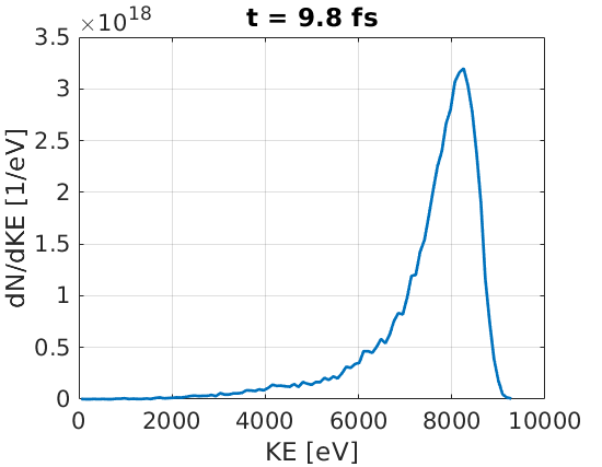
The average energy of incident electrons was found to be 7.5 keV, which is close to the estimated value. An exact fit is not expected, as rates and kinematics change as ionisation events modify the incident electron energies.

These plots were produced using the input deck below:

begin:control
  nx = 500
  x_min = 0
  x_max = 5.0e-6
  t_end = 10.0e-15
  verbose = 2
  stdout_frequency = 1
end:control

begin:boundaries
  bc_x_min = periodic
  bc_x_max = periodic
end:boundaries

begin:physics_package
  process = collision_ionise_recombine
  incident = Electron
  background = Copper
  ionise_to_species = Copper1
  ejected_electron = Ejected_electron
end:physics_package

begin:species
  name = Electron
  mass = 1
  charge = 0
  drift_x = 5.4291e-23
  rho = 1.0e27
  npart = 50 * nx
end:species

begin:species
  name = Copper
  atomic_number = 29
  charge = 0
  mass = 116595.7
  rho = 6.0e28
  npart_per_cell = 1000
  immobile = T
end:species

begin:species
  name = Copper1
  atomic_number = 29
  charge = 1
  mass = 116595.7 - 1
  immobile = T
end:species

begin:species
  name = Ejected_electron
  immobile = T
  identify:electron
end:species

begin:output
  name = rst
  nstep_snapshot = 10
  rolling_restart = F
  dump_first = T
end:output

Number density evolution

The Python script used to plot the number density evolution is provided here:

import sys
sys.path.append('/home/stuart/Postdoc/EPOCpp/epc_readers')

from epc_parser import epc
import numpy as np
import matplotlib.pyplot as plt

core_count = 1
start_file_no = 0
end_file_no = 310
file_no_spacing = 10
spec_id = 1
path_to_data = "/home/stuart/Postdoc/EPOCpp/example_decks/Physics_package_examples/"

# Obtain x positions of all particles
x_data = np.array([])
i_plot = 0
arr_size = int((end_file_no - start_file_no)/file_no_spacing + 1)
density = np.empty(arr_size)
time = np.empty(arr_size)
for file_no in range(start_file_no, end_file_no + file_no_spacing, file_no_spacing):
  file_no_string = str(file_no).zfill(5)
  if (core_count > 1):
    for i in range(core_count):
      core_str = str(i).zfill(3)
      print(core_str)
      data = epc(path_to_data + "data" + file_no_string + "_" + core_str + ".epc")
      print(path_to_data + "data" + file_no_string + "_" + core_str + ".epc")
      x_data = np.concatenate((x_data, data.get_array("/data/" + str(file_no) + "/particles/" + str(spec_id) + "/position/x")))
  else:
    data = epc(path_to_data + "data" + file_no_string + ".epc")
    x_data = data.get_array("/data/" + str(file_no) + "/particles/" + str(spec_id) + "/position/x")
    print(path_to_data + "data" + file_no_string + ".epc")

  
  # Domain-averaged number density  
  w_data = data.get_array("/data/" + str(file_no) + "/particles/" + str(spec_id) + "/weighting")
  [x_min, x_max] = data.get_array("/data/" + str(file_no) + "/meshes/attributes/extents")
  density[i_plot] = x_data.size * w_data / (x_max - x_min)
  time[i_plot] = data.get_array("/data/" + str(file_no) + "/attributes/time")[0]
  i_plot = i_plot + 1

# Create plot
plt.plot(time, density)
plt.xlabel('t [s]', fontsize=16)
plt.ylabel('Number density [1/m³]', fontsize=16)
plt.grid(True, which='both', linestyle='--', linewidth=0.5, alpha=0.7)
plt.xticks(fontsize=14)
plt.yticks(fontsize=14)

np.savetxt("x_vals.txt", time)
np.savetxt("y_vals.txt", density)

# Show the plot
plt.show()