
Example 1: Basic sampling#
These examples showcase the most basic setup for the physics package interface.
They use the physics package test_process_single, which has a constant trigger
rate of 1.0e8/s for all incident particles. When triggered, the process simply
sets the incident particle momentum to zero.
In these examples, 1e5 electrons are loaded into the cell on the x_min
boundary, with a highly relativistic drift momentum. The number density is
sufficiently low to prevent the generation of fields which significantly affect
the electron trajectories.
Three example decks have been provided for this system, demonstrating different sampling behaviours:
example_1_0: The default sampler settings are usedexample_1_1: Super-cycling is used, reducing the number of times the package is runexample_1_2: The process rate is artificially modified from the input deck
Example 1.0#
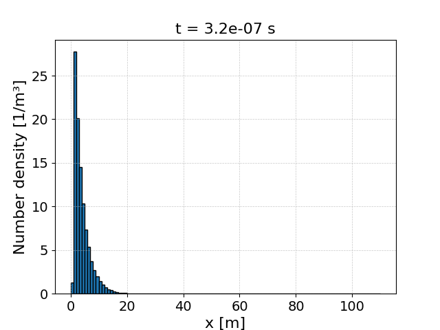
The electrons travel relativistically until the process is triggered, and since the process rate is constant, the distances reached by each electron will follow an exponential distribution. Sampling in the default scheme is performed using the optical depth method, where a permanent MPI-aware particle variable is created for each incident particle, which determines how far the particle travels through a target (or laser or vacuum) before the process is triggered. This optical depth only needs to be sampled once per particle, and is only re-sampled after the process triggers.
The physics package block takes the form:
begin:physics_package
   process = test_process_single
   incident = Electron_bunch
end:physics_package
And the final spatial distribution does indeed follow an exponential profile:
Example 1.1#
In this example, the optical depth is only updated once every 2nd step. This update uses a time-step twice as large as the simulation time-step to compensate, and should result in particles reaching the same depth as in Example 1.0.
This uses the physics package block:
begin:physics_package
   process = test_process_single
   incident = Electron_bunch
   run_on_nth = 2
end:physics_package
And yields:
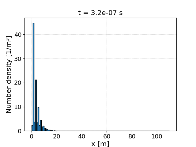
The behaviour is similar to before, but with some differences. Because each
particle starts in the same cell, and only travels one cell per time-step, then
the process won’t run when most particles are in every-other cell. This leads to
the high-low-high densities seen here. While super-cycling requires fewer
evaluations of physics packages, it comes at a cost of reduced temporal
resolution in the physics packages. For processes which occur rapidly like
test_process_single, artefacts like those seen here are to be expected.
Example 1.2#
When investigating the code itself, it may be helpful to modify the physics
package rates from the input deck. This can be done using the
artificial_rate_boost key. The term “artificial” is used, as modifying the
rates like this will make the simulation non-physical. This is also to
distinguish it from other rate-boosting effects like super-cycling or secondary
particle re-sampling, which shouldn’t affect the physical result.
This can be run using the physics package block:
begin:physics_package
   process = test_process_single
   incident = Electron_bunch
   artificial_rate_boost = 0.2
end:physics_package
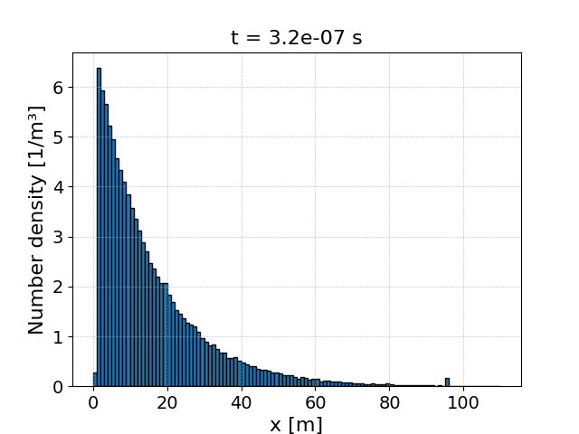
Here the rate has been reduced by a factor of 5, which should allow the incident electrons to travel further before the process triggers and they stop. This is what is seen when the simulation is run:
1D density plotter#
The python script used to generate the figures in this section is given here:
import sys
sys.path.append('/home/stuart/Postdoc/EPOCpp/epc_readers')

from epc_parser import epc
import numpy as np
import matplotlib.pyplot as plt

core_count = 4
file_no = 100
spec_id = 3
path_to_data = "/home/stuart/Postdoc/Keith/EPOCpp/example_decks/Physics_package_examples/"

file_no_string = str(file_no).zfill(5)

# Obtain x positions of all particles
x_data = np.array([])
if (core_count > 1):
  for i in range(core_count):
    core_str = str(i).zfill(3)
    print(core_str)
    data = epc(path_to_data + "data" + file_no_string + "_" + core_str + ".epc")
    print(path_to_data + "data" + file_no_string + "_" + core_str + ".epc")
    x_data = np.concatenate((x_data, data.get_array("/data/" + str(file_no) + "/particles/" + str(spec_id) + "/position/x")))
else:
  data = epc(path_to_data + "data" + file_no_string + ".epc")
  x_data = data.get_array("/data/" + str(file_no) + "/particles/" + str(spec_id) + "/position/x")

# Obtain x grid
[x_min, x_max] = data.get_array("/data/" + str(file_no) + "/meshes/attributes/extents")
nx = data.get_array("/data/" + str(file_no) + "/meshes/attributes/cells")
dx = (x_max - x_min) / nx
x_edges = np.linspace(x_min, x_max, nx[0] + 1)

# Number of particles in each cell
counts, _ = np.histogram(x_data, bins=x_edges)

# Scaled number density
w_data = data.get_array("/data/" + str(file_no) + "/particles/" + str(spec_id) + "/weighting")
num_dens = counts * w_data / dx

# Create plot
x_centres = 0.5 * (x_edges[:-1] + x_edges[1:])
plt.bar(x_centres, num_dens, width=np.diff(x_edges), align='center', edgecolor='k')
plt.xlabel('x [m]', fontsize=16)
plt.ylabel('Number density [1/m³]', fontsize=16)
plt.grid(True, which='both', linestyle='--', linewidth=0.5, alpha=0.7)
plt.xticks(fontsize=14)
plt.yticks(fontsize=14)
time = data.get_array("/data/" + str(file_no) + "/attributes/time")[0]
t_string = f"{time:.1e}"
plt.title(f"t = {t_string} s", fontsize=16)

# Show the plot
plt.show()