Example 4: Particle background

Some physics packages involve interaction with a background species, but don’t significantly modify the properties of background particles themselves. These packages are often described with a cross-section, and require the incident particle speed and the background number density to get a trigger-rate.

The physics package test_process_Z_background demonstrates this kind of interaction. The process has a constant cross-section of 1.0e-3 m², and accepts background species as arguments. Upon trigger, the incident electron momentum \(p_x\) is set to zero. Multiple backgrounds may be specified, provided they all represent the same type of particle. For multiple different backgrounds, the processes must be setup separately.

These examples have a similar setup to Example 1, where a relativistic, low-density electron bunch passes through the simulation window. A static background of electrons is also present, which acts as the background species for the test_process_Z_background interaction.

Four examples are provided for this system:

• example_4_0: Default settings

• example_4_1: Two equivalent background species are used

• example_4_2: Two processes are used, with a shared background

• example_4_3: The background number density is saved, and updated less often

Example 4.0

The incident electrons start in the first cell, and move across the domain at relativistic speed. A uniform density of background particles is present, and the cross-section of test_process_Z_background is also constant - hence, the trigger rate is fixed for electrons in the incident species.

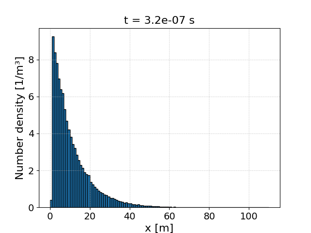
Upon trigger, the incident electron has its \(p_x\) set to 0, and will remain at the trigger location. Since the rate of trigger is constant, the density distribution is expected to form an exponential decay.

The physics package block takes the form:

begin:physics_package
   process = test_process_Z_background
   incident = Electron_bunch
   background = Background_electrons
end:physics_package

The density at the end of the simulation is as expected:

Example 4.1

This example also uses test_process_Z_background, with a constant cross-section, and a uniform background density. This time, two equivalent background densities are used.

In this case, the code can sum the number densities, and sample the process once with a combined density. This is an improvement on the FORTRAN code, where the trigger-test would be performed for each background separately, causing unnecessary computation.

The physics package block setup for this example is:

begin:physics_package
   process = test_process_Z_background
   incident = Electron_bunch
   background = Background_electrons
   background = Background_electrons2
end:physics_package

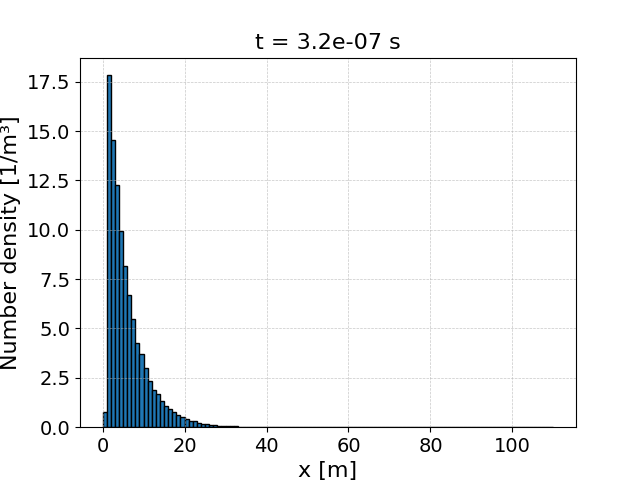
Background_electrons has the same number density as in Example 4.0, and Background_electrons2 also has this density. Hence, since the number of target particles has doubled, the trigger rate has also doubled. This can be seen with the faster exponential decay in this simulation:

Example 4.2

Instead of using one process with two identical backgrounds as in Example 4.1, here we create an equivalent system where two processes act on the same background. The code will only calculate the background number density once per step, and both processes will use this background array.

This uses the physics package block:

begin:physics_package
   process = test_process_Z_background
   incident = Electron_bunch
   background = Background_electrons
end:physics_package

begin:physics_package
   process = test_process_Z_background
   incident = Electron_bunch
   background = Background_electrons
end:physics_package

This setup is physically equivalent to Example 4.1, and we get the same exponential decay pattern in the number density.

Example 4.3

In this example, a single test_process_Z_background is used with a single background species, but the background number density is only calculated once every 1.0e-7s in the simulation. The number density array is saved between these calculations, which prevents re-calculating the density each step. This feature is useful to reduce computational expense in systems where the number density of background particles changes slowly.

Background array super-cycling was switched on using this physics package block:

begin:physics_package
   process = test_process_Z_background
   incident = Electron_bunch
   background = Background_electrons
   recalc_time_num_density = 1.0e-7
end:physics_package

As this example is physically equivalent to Example 4.0, it is good to see we get the same density profile: