Bremsstrahlung

Bremsstrahlung refers to the radiation which is produced when an incident particle undergoes acceleration in the Coulomb field of a target nucleus. The bremsstrahlung process may be modelled classically following Jackson’s “Classical Electrodynamics” textbook, or Sections 2.2-2.2.3 and 4.5.2 in the thesis of Morris (2021) “High energy X-ray production in laser-solid interactions”. While classical descriptions lack a full physical treatment, they can be useful in deriving general scaling laws.

For example, in electron bremsstrahlung, the stopping power \(d\epsilon/dx\) takes the form:

\(\frac{d\epsilon}{dx} \approx 3\times 10^{-31} \epsilon n_i Z^2 \ln\left(192 Z^{-1/3}\right)\)

where \(\epsilon\) is the total electron energy, \(n_i\) is the background ion density, \(Z\) is the ion atomic number, and all terms are evaluated in SI units. Hence, we may expect the electron energy loss due to bremsstrahlung radiation to scale roughly with \(Z^2\).

Cross sections

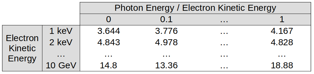
The full bremsstrahlung cross sections including quantum corrections for neutral targets are tabulated by Seltzer and Berger (Atomic data and nuclear data tables, 35(3), 345-418 (1986)). These tables give the differential cross section:

\(\left(\frac{\beta_e}{Z}\right)^2 E_\gamma \frac{d\sigma}{d E_\gamma}\)

where \(\beta_e\) is the electron velocity normalised to the speed of light \(v_e/c\), \(E_\gamma\) is the photon energy, and \(d\sigma/d E_\gamma\) is the differential cross section. These quantities are quoted in millibarns, and some values for the Al table are given below:

In this raw form, the tables aren’t suitable for EPOCH modelling. We require a total cross-section \(\sigma\) to determine when photons are emitted, and a cumulative distribution function \(F(E_\gamma)\) for sampling photon energies.

Here, \(\sigma\) can be calculated from:

\(\sigma = \int_{E_{\gamma,\text{cut}}}^{\epsilon_k} \frac{d\sigma}{d E_\gamma} d E_\gamma\)

for electrons of kinetic energy \(\epsilon_k\). Note that as \(E_\gamma \rightarrow 0\), \(d\sigma / dE_\gamma \rightarrow \infty\), as the formula allows an infinite number of zero-energy photons to be produced. Such a scheme would make sampling bremsstrahlung pointless, as we would simply radiate an infinite amount of insignificant photons, and never sample an important photon. Instead, we only consider photon energies down to \(E_{\gamma,\text{cut}}\), which is defined such that the energy carried by photons below this energy only accounts for fraction \(10^{-9}\) of the total emission:

\(\int_0^{E_{\gamma,\text{cut}}} E_\gamma \frac{d \sigma}{dE_\gamma} dE_\gamma = 10^{-9}\int_0^{\epsilon_k} E_\gamma \frac{d \sigma}{dE_\gamma} dE_\gamma\)

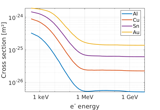
This yields total bremsstrahlung cross sections as a function of incident electron kinetic energy, which appear as

Photon sampling

For sampling photon energies, a cumulative distribution function \(F(E_\gamma)\) is calculated using

\(F(E_\gamma) = \frac{1}{\sigma}\int_{E_{\gamma,\text{cut}}}^{E_\gamma} \frac{d\sigma}{d E_\gamma'}dE_\gamma'\)

Hence, for each \(\epsilon_k\), a range of \(E_\gamma\) values are considered from \(E_{\gamma,\text{cut}}\) to \(\epsilon_k\), and the CDF \(F(E_\gamma)\) is calculated for each one. When sampling photon energies, a random number is calculated for the CDF, and the corresponding \(E_\gamma\) value is interpolated from the \(E_\gamma\) lists at the neighbouring \(\epsilon_k\) evaluation points for the current incident electron. An example of the EPOCH table format is given below:

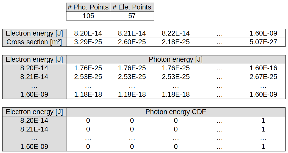
Note that the greyed-out cells have been included to demonstrate the format of the tables, but these are not present in the actual bremsstrahlung table files.

Plasma-screening

The Seltzer-Berger cross sections describe bremsstrahlung radiation due to electrons interacting with neutral background particles, including quantum effects. However, PIC codes often deal with targets heated to a plasma state, and the Debye-screening of a nucleus in a plasma is different from the atomic-screening of orbital electrons. Users may optionally switch on a “plasma-screening” model to correct for this.

This model is described in the Morris (2021) thesis Section 4.5.2, and is based off an interpolation between the atomic-screened and Debye-screened classical bremsstrahlung radiation cross-section:

\(E_\gamma\frac{d\sigma}{d E_\gamma} \propto \left(Z^*\right)^2 \left( \left(\frac{Z}{Z^*} \right)^2 \ln\left| \frac{a m_e v_e}{\hbar}\right| + \ln\left| \frac{\lambda_D}{a} \right| \right)\)

where \(Z^*\) is the ion charge-state, \(a = 1.4 a_B Z^{-1/3}\) for Bohr radius \(a_B\), and \(\lambda_D\) is the plasma Debye length. This equation yields the atomic-screened case for \(Z^* = 0\), and the Debye-screened case for \(Z^* = Z\).

In the EPOCH model, this approximation is used to derive a “plasma enhancement factor” \(F_\sigma\), which is the ratio of the general radiation cross-section to the atomic radiation cross-section:

\(F_\sigma = \frac{\left. E_\gamma d\sigma /d E_\gamma \right|_{Z^*}}{\left. E_\gamma d\sigma /d E_\gamma \right|_{Z^*=0}}\)

or, following equation (B3) in Morris (2021) Phys. of Plasmas, 28(10):

\(F_\sigma = 1 + \frac{\ln\left|\lambda_D/a\right|}{\ln\left|am_e c/\hbar\right|}\)

where the electron speed is evaluated in the relativistic limit \(v_e=c\), and we have corrected a typo in (B3) to make the denominator dimensionally correct.

Angular distribution

In the ultra-relativistic limit, the angular distribution of photon emission becomes strongly peaked in the incident electron direction, which is the default emission mode for EPOCH.

The user also has the option to sample photon emission direction from an approximate fit to the angular distribution of bremsstrahlung radiation. In EPOCH, this fit uses the Geant4 model for the probability distribution function \(f(\gamma\theta)\):

\(f(\gamma\theta) = \frac{a^2\gamma\theta}{4}\left( e^{-a\gamma\theta} + 27e^{-3a\gamma\theta} \right)\)

where \(\theta\) is the angle between the electron and photon momenta at the time of emission, \(\gamma\) is the electron Lorentz factor, and the fit parameter \(a = 0.625\). The azimuthal rotation angle \(\phi\) is sampled uniformly from 0 to \(2\pi\), and \(\theta\) will only be accepted between 0 and \(\pi\).

The PDF \(f(\gamma\theta)\) is only an approximate PDF, as it is not normalised between the limits of \(\theta\). Sampling proceeds as described by the Geant4 Physics Reference Manual:

• Generate 3 uniformly distributed random numbers between 0 and 1: \(r_1\), \(r_2\), \(r_3\)

• If \(r_1 < 0.25\), \(b = 0.625\), otherwise \(b = 1.875\)

• \(\theta = - \ln(r_2 r_3) / \gamma b\)

• If \(\theta < \pi\), accept sample, otherwise start again

Positron bremsstrahlung

EPOCH is also capable of modelling bremsstrahlung radiation from positrons. The difference between the bremsstrahlung stopping powers of electrons and positrons has been recorded in Table II of Kim, L., et al (1986). Phys. Rev. A, 33(5), 3002. The tabulated values vary as a function of the ratio of incident particle kinetic energy to the atomic number squared, and take the form:

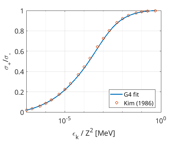
Here, we equate the ratio in stopping power to the ratio of total bremsstrahlung cross-sections. A fit to the tabulated values is taken from the Geant4 Physics Reference Manual, and is plotted over the data-points above.

The fit uses the parameter:

\(t = ln\left(1 + \frac{10^6 \gamma_e}{Z^2} \right)\)

where \(\gamma_e\) is the relativistic Lorentz factor for the particle. The Geant4 fit model takes the form:

\(\frac{\sigma_+}{\sigma_-} = 1 - \exp\left(-0.12359t + 0.061274t^2 - 0.031516t^3 + 0.0077446t^4 ...\right.\) \( ... \left. - 0.0010595t^5 + 7.0568\times 10^{-5}t^6 - 1.8080\times 10^{-6}t^7\right)\)

Example: Basic

In this example, \(5 \times 10 ^5\) electrons are loaded uniformly into the first 5 cells of a 1D simulation domain. A drift momentum of \(5.344\times 10^{-19}\) kgm/s is applied, equivalent to a kinetic energy of 1 GeV. These electrons traverse a 5.5 mm solid-density Al target, and electron bremsstrahlung is switched on.

The bremsstrahlung cross section for 1 GeV electrons in Al is \(5.2\times 10^{-27}\) m², the electron speed is roughly \(c\), and the Al number density is \(6.0\times 10^{28}\)/m³. This implies a bremsstrahlung radiation rate of \(9.4\times 10^{10}\)/s. If we assume that photon emission energies for 1 GeV electrons are negligible compared to the electron energy, then the emission rate will not change much after repeated photon emission. This allows us to estimate the time each electron spends in a cell, and the number density of photons produced over that time.

This theory density can be compared to the number density of created photons in the EPOCH simulation if the photon macro-particles are kept immobile. This comparison has been shown here:

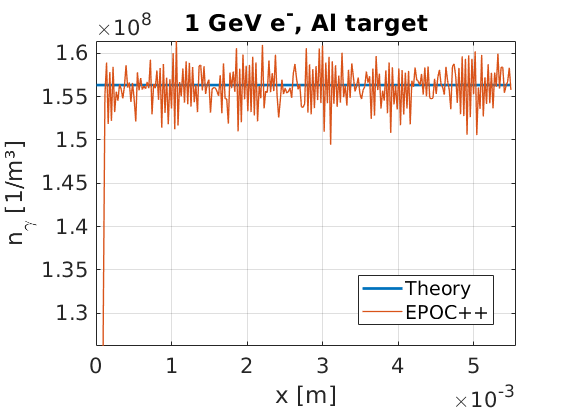
As can be seen, the number density of bremsstrahlung photon creation sites is uniform over the simulation domain, and there is good agreement between theory and simulation.

The photon energy spectrum can be compared to the spectrum expected from the CDF for 1 GeV electrons in Al, and also shows the expected behaviour:

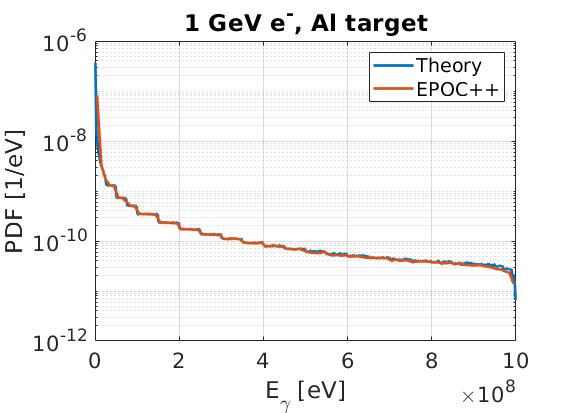
The stepping pattern in this figure is a result of how interpolation is performed between evaluation points in the bremsstrahlung tables. A linear interpolation, when viewed on a log-scale, will feature this artefact.

The input deck used to generate these figures is given here:

begin:control
  nx = 256
  x_min = 0
  x_max = 5.50e-3
  t_end = 2.0e-11
  verbose = 2
  stdout_frequency = 10
end:control

begin:boundaries
  bc_x_min = open
  bc_x_max = open
end:boundaries

begin:physics_package
  process = bremsstrahlung
  incident = Electron_bunch
  background = Aluminium
  photon_species = Photon
  min_secondary_energy = 0
end:physics_package

begin:species
  name = Electron_bunch
  drift_x = 5.344e-19
  rho = 1.0e5 * nx / (x_max - x_min)
  rho = if (x lt 5*dx, density(Electron_bunch), 0)
  npart = 2048000
  identify:electron
end:species

begin:species
  name = Aluminium
  atomic_number = 13
  charge = 0
  mass = 49218
  rho = 6.022e28
  npart_per_cell = 2000
  immobile = T
end:species

begin:species
  name = Photon
  immobile = T
  identify:photon
end:species

begin:output
  name = rst
  nstep_snapshot = 10
  rolling_restart = F
  dump_first = T
end:output

Example: Plasma-screening

Like the previous section, this example also features a 1 GeV electron beam of \(5\times 10^5\) particles, but this time, the target is composed of \(\text{Al}^{12+}\) ions heated to 1 keV, and the plasma-screening model is switched on.
In this setup, we have \(F_\sigma \approx 1.2\), which results in the following photon number densities:

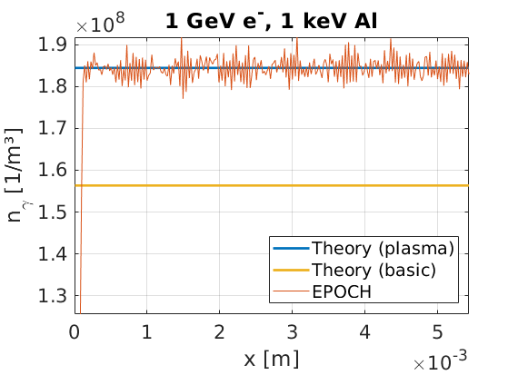
Photon macro-particles are made immobile such that these number densities refer to photon creation sites, and theory curves with and without the plasma screening factor have been included using the known Al cross-sections. This simulation was performed using the following input deck:

begin:control
  nx = 256
  x_min = 0
  x_max = 5.50e-3
  t_end = 2.0e-11
  verbose = 2
  stdout_frequency = 10
end:control

begin:boundaries
  bc_x_min = open
  bc_x_max = open
end:boundaries

begin:physics_package
  process = bremsstrahlung
  incident = Electron_bunch
  background = Aluminium
  photon_species = Photon
  min_secondary_energy = 0
  use_brem_plasma_screening = T
end:physics_package

begin:species
  name = Electron_bunch
  drift_x = 5.344e-19
  rho = 1.0e5 * nx / (x_max - x_min)
  rho = if (x lt 5*dx, density(Electron_bunch), 0)
  npart = 2048000
  identify:electron
end:species

begin:species
  name = Aluminium
  atomic_number = 13
  charge = 12
  temp_ev = 1.0e3
  mass = 49218
  rho = 6.022e28
  npart_per_cell = 2000
  immobile = T
end:species

begin:species
  name = Photon
  immobile = T
  identify:photon
end:species

begin:output
  name = rst
  nstep_snapshot = 10
  rolling_restart = F
  dump_first = T
end:output

Example: Angular distribution

This example tracks the angular distribution of radiated photons, compared to the Geant4 sampling method. An electron bunch of \(5\times 10^{5}\) electrons with kinetic energy around 25 MeV pass through an Al target, in a simulation with the sample_angular_dist key switched on. The electrons were initialised with momentum in the positive \(x\)-direction only, so \(\theta\) refers to the deviation of the photon momentum to this initial electron direction. The resultant plot is given here:

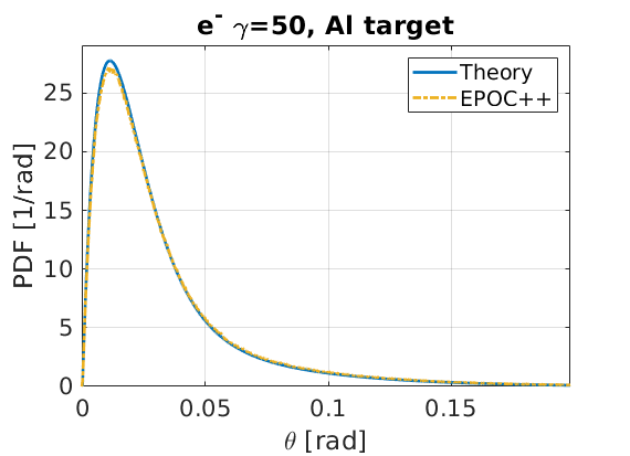
Note that for the comparison to theory, the Geant4 \(f(\gamma\theta)\) has been scaled such that it becomes normalised between \(\theta=0\) and \(\theta=\pi\). The simulation in this figure used the following input deck:

begin:control
  nx = 256
  x_min = 0
  x_max = 5.50e-3
  t_end = 2.0e-11
  verbose = 2
  stdout_frequency = 10
end:control

begin:boundaries
  bc_x_min = open
  bc_x_max = open
end:boundaries

begin:physics_package
  process = bremsstrahlung
  incident = Electron_bunch
  background = Aluminium
  photon_species = Photon
  min_secondary_energy = 0
  sample_angular_dist = T
end:physics_package

begin:species
  name = Electron_bunch
  drift_x = 1.37e-20
  rho = 1.0e5 * nx / (x_max - x_min)
  rho = if (x lt 5*dx, density(Electron_bunch), 0)
  npart = 2048000
  identify:electron
end:species

begin:species
  name = Aluminium
  atomic_number = 13
  charge = 0
  mass = 49218
  rho = 6.022e28
  npart_per_cell = 2000
  immobile = T
end:species

begin:species
  name = Photon
  immobile = T
  identify:photon
end:species

begin:output
  name = rst
  nstep_snapshot = 10
  rolling_restart = F
  dump_first = T
end:output

Example: Positron bremsstrahlung

To demonstrate the differences between positron and electron bremsstrahlung radiation, this example will fire two bunches through a 0.55mm gold target. Both bunches start in the 5 cells next to the x_min boundary, contain \(5\times 10^5\) particles, and have energies around 62 MeV. One bunch contains electrons and the other contains positrons, and both bunches have their own photon species to populate with radiated macro-particles. This separation of photons will allow us to determine which photons were radiated by electrons, and which were from positrons.

In this example, the electron bremsstrahlung cross section is around \(1.4\times 10^{-25}\) m², and the cross section ratio is around \(\sigma_+/\sigma_- \approx 0.92\). This results in a difference between the electron and positron radiation, which is shown here:

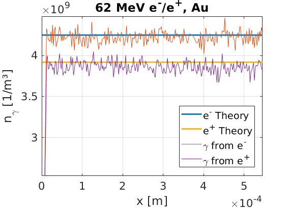
This plot demonstrates good agreement with the simulation results, and the expected photon distributions from the known rates of radiation. The input deck used to create the data in this figure is given here:

begin:control
  nx = 256
  x_min = 0
  x_max = 5.50e-4
  t_end = 2.0e-12
  verbose = 2
  stdout_frequency = 10
end:control

begin:boundaries
  bc_x_min = open
  bc_x_max = open
end:boundaries

begin:physics_package
  process = bremsstrahlung
  incident = Electron_bunch
  background = Gold
  photon_species = Photon_from_ele
  min_secondary_energy = 0
end:physics_package

begin:physics_package
  process = bremsstrahlung
  incident = Positron_bunch
  background = Gold
  photon_species = Photon_from_pos
  min_secondary_energy = 0
end:physics_package

begin:species
  name = Electron_bunch
  drift_x = 3.3e-20
  rho = 1.0e5 * nx / (x_max - x_min)
  rho = if (x lt 5*dx, density(Electron_bunch), 0)
  npart = 204800
  identify:electron
end:species

begin:species
  name = Positron_bunch
  drift_x = 3.3e-20
  rho = 1.0e5 * nx / (x_max - x_min)
  rho = if (x lt 5*dx, density(Electron_bunch), 0)
  npart = 204800
  identify:positron
end:species

begin:species
  name = Gold
  atomic_number = 79
  charge = 0
  mass = 359109
  rho = 6.022e28
  npart_per_cell = 2000
  immobile = T
end:species

begin:species
  name = Photon_from_ele
  immobile = T
  identify:photon
end:species

begin:species
  name = Photon_from_pos
  immobile = T
  identify:photon
end:species

begin:output
  name = rst
  nstep_snapshot = 10
  rolling_restart = F
  dump_first = T
end:output

Python energy spectrum plotter

import sys
sys.path.append('/home/stuart/Postdoc/EPOCpp/epc_readers')

from epc_parser import epc
import numpy as np
import matplotlib.pyplot as plt

core_count = 1
file_no = 400
spec_id = 3
path_to_data = "/home/stuart/Postdoc/Keith/EPOCpp/example_decks/Physics_package_examples/"

file_no_string = str(file_no).zfill(5)

# Obtain x positions of all particles
px_data = np.array([], dtype=float)
py_data = np.array([], dtype=float)
pz_data = np.array([], dtype=float)
if (core_count > 1):
  for i in range(core_count):
    core_str = str(i).zfill(3)
    print(core_str)
    data = epc(path_to_data + "data" + file_no_string + "_" + core_str + ".epc")
    px_data = np.concatenate((px_data, data.get_array("/data/" + str(file_no) + "/particles/" + str(spec_id) + "/momentum/x")))
    py_data = np.concatenate((py_data, data.get_array("/data/" + str(file_no) + "/particles/" + str(spec_id) + "/momentum/y")))
    pz_data = np.concatenate((pz_data, data.get_array("/data/" + str(file_no) + "/particles/" + str(spec_id) + "/momentum/z")))
else:
  data = epc(path_to_data + "data" + file_no_string + ".epc")
  px_data = data.get_array("/data/" + str(file_no) + "/particles/" + str(spec_id) + "/momentum/x")
  py_data = data.get_array("/data/" + str(file_no) + "/particles/" + str(spec_id) + "/momentum/y")
  pz_data = data.get_array("/data/" + str(file_no) + "/particles/" + str(spec_id) + "/momentum/z")

# Obtain x grid
p2 = np.square(px_data) + np.square(py_data) + np.square(pz_data)
c = 299792458
q0 = 1.60217663e-19
m = data.get_array("/data/" + str(file_no) + "/particles/" + str(spec_id) + "/mass")
E2 = np.array(p2 * c * c + m * m * pow(c, 4), dtype=float)
ke_ev = (np.sqrt(E2) - m*c*c) / q0  

# Number of particles in each cell
counts, bin_edges = np.histogram(ke_ev, 100)
dE = bin_edges[1]-bin_edges[0]

# Scaled number density
w_data = data.get_array("/data/" + str(file_no) + "/particles/" + str(spec_id) + "/weighting")
dN_dE = counts * w_data / dE

# Create plot
x_centres = 0.5 * (bin_edges[:-1] + bin_edges[1:])
plt.bar(x_centres, dN_dE, width=np.diff(bin_edges), align='center', edgecolor='k')
plt.xlabel('KE [eV]', fontsize=16)
plt.ylabel('dN/dKE [1/eV]', fontsize=16)
plt.grid(True, which='both', linestyle='--', linewidth=0.5, alpha=0.7)
plt.xticks(fontsize=14)
plt.yticks(fontsize=14)
time = data.get_array("/data/" + str(file_no) + "/attributes/time")[0]
t_string = f"{time:.1e}"
plt.title(f"t = {t_string} s", fontsize=16)

np.savetxt("x_vals.txt", bin_edges)
np.savetxt("y_vals.txt", dN_dE)

# Show the plot
plt.show()

Python angular distribution plotter

import sys
sys.path.append('/home/stuart/Postdoc/EPOCpp/epc_readers')

from epc_parser import epc
import numpy as np
import matplotlib.pyplot as plt

core_count = 1
file_no = 400
spec_id = 3
path_to_data = "/home/stuart/Postdoc/Keith/EPOCpp/example_decks/Physics_package_examples/"

file_no_string = str(file_no).zfill(5)

# Obtain x positions of all particles
px_data = np.array([], dtype=float)
py_data = np.array([], dtype=float)
pz_data = np.array([], dtype=float)
if (core_count > 1):
  for i in range(core_count):
    core_str = str(i).zfill(3)
    print(core_str)
    data = epc(path_to_data + "data" + file_no_string + "_" + core_str + ".epc")
    px_data = np.concatenate((px_data, data.get_array("/data/" + str(file_no) + "/particles/" + str(spec_id) + "/momentum/x")))
    py_data = np.concatenate((py_data, data.get_array("/data/" + str(file_no) + "/particles/" + str(spec_id) + "/momentum/y")))
    pz_data = np.concatenate((pz_data, data.get_array("/data/" + str(file_no) + "/particles/" + str(spec_id) + "/momentum/z")))
else:
  data = epc(path_to_data + "data" + file_no_string + ".epc")
  px_data = data.get_array("/data/" + str(file_no) + "/particles/" + str(spec_id) + "/momentum/x")
  py_data = data.get_array("/data/" + str(file_no) + "/particles/" + str(spec_id) + "/momentum/y")
  pz_data = data.get_array("/data/" + str(file_no) + "/particles/" + str(spec_id) + "/momentum/z")

# Obtain x grid
theta = np.arctan(np.sqrt(np.square(py_data) + np.square(pz_data)) / px_data) 

# Number of particles in each cell
counts, bin_edges = np.histogram(theta, 10000)
dth = bin_edges[1]-bin_edges[0]

# Scaled number density
w_data = data.get_array("/data/" + str(file_no) + "/particles/" + str(spec_id) + "/weighting")
dN_dth = counts * w_data / dth

# Create plot
x_centres = 0.5 * (bin_edges[:-1] + bin_edges[1:])
plt.bar(x_centres, dN_dth, width=np.diff(bin_edges), align='center', edgecolor='k')
plt.xlabel('Theta [rad]', fontsize=16)
plt.ylabel('dN/dtheta [1/rad]', fontsize=16)
plt.grid(True, which='both', linestyle='--', linewidth=0.5, alpha=0.7)
plt.xticks(fontsize=14)
plt.yticks(fontsize=14)
time = data.get_array("/data/" + str(file_no) + "/attributes/time")[0]
t_string = f"{time:.1e}"
plt.title(f"t = {t_string} s", fontsize=16)

np.savetxt("x_vals.txt", bin_edges)
np.savetxt("y_vals.txt", dN_dth)

# Show the plot
plt.show()